Abstract: Queueing models in which customers or messages arrive in batches with inter-arrival times of batches possibly correlated and services rendered in batches of varying sizes play an important role in telecommunication systems. Recently queueing models of BMAP/G/1-type in which a new type of group clearance was studied using embedded Markov renewal process as well as continuous time Markov chain whose generator has a very special structure. In this paper, we generalize these models to multi-server systems through simulation approach. After validating the simulation model for the single server case, we report our simulated results for much more general situations.
Index Terms: Desktop Grid, Multiserver Systems, Group Clearance, BMAP, Simulation.
I. INTRODUCTION
Queueing models in which arrivals and services occur in batches have been studied extensively in the literature (see e.g., [6]). Recently, a queueing model in which arrivals occur according to a batch Markovian arrival process (BMAP), a versatile point process introduced by Neuts [10]. The services are offered in groups of varying sizes such that all waiting customers at the beginning of a service are taken into service, was studied by Chakravarthy, et.al., [5]. This type of group services was first studied in [5]. Such models, referred to as queueing models with group clearance in [5], have applications in modern telecommunication and computing
systems, such as distributed and cloud computing, data transfer by means of wireless networks, solid-state drives and many other applications, thanks to recent developments in information technology. The authors in [5] employ matrix-analytic methods and report some interesting results both analytically and numerically by looking at the model in the context of a single server. Illustrative numerical examples are based on service times with phase type distribution. In the present paper we extend the aforementioned models to multi-server systems. While one can study the multi-multi-server systems along the lines of [5], here we will resort to simulation to study such systems.
Revised Manuscript Received on May 28, 2019.
Srinivas R. Chakravarthy, Departments of Industrial and Manufacturing Engineering & Mathematics, Kettering University,Flint, MI-48504, USA; [email protected]
Alexander Rumyantsev, Institute of Applied Mathematical Research, Karelian Research Centre of RAS, Petrozavodsk, Russia; Petrozavodsk State University, Petrozavodsk, Russia; [email protected].
Suppose that generator 𝑄 = ∑∞𝑘=0𝐷𝑘 of dimension m is an irreducible generator of a continuous-time Markov chain (CTMC) such that D0 governs transitions corresponding to no arrivals/events to a system, and Dk governs transitions corresponding arrivals of size k, k ≥ 1. A BMAP is now formally characterized by the sequence of matrices {Dk}. The point process of BMAP is a semi-Markov process with transition probability matrix given by
∫ 𝑒𝑥 𝐷0𝑡𝑑𝑡
0 = [𝐼 − 𝑒
𝐷0𝑥](−𝐷
0)−1 𝐷𝑘, 𝑘 ≥ 1. (1)
One can choose the initial probability vector, α, of the CTMC with generator Q, in a variety of ways to make the BMAP to be even more suitable for many applications in practice. Among the many choices, the most interesting one is α = π, where πQ = 0, πe = 1, where e is a column vector of dimension m with all entries equal to 1.
The fundamental rate, λ, is defined as λ = π∑∞𝑘=1𝑘𝐷𝑘𝒆. The quantity λ gives the rate (per unit of time) at which customers arrive to the system. The quantity λg = π (−D0) e gives the rate (per unit of time) at which batches arrive to the system. To have a specific value for λgwe multiply the Dk, k ≥ 0, by the appropriate common constant.
The motivation for Neuts to introduce BMAP as a versatile Markovian point process is the ability to model correlation, if any, of successive inter-arrival times and at the same time use matrix algebra to carry out the analysis of queueing models involving such processes. For full details on BMAP and its special cases including applications and reviews, we refer to [1–3, 8, 9, 12, 13].
Very briefly the model studied in [5] is as follows. Customers arrive according to a BMAP. If the arriving batch of customers finds the server idle, the entire batch gets into service; otherwise, the batch gets into a buffer (with unlimited capacity). The service times are generally distributed but for illustrative examples, the authors use phase type (PH-) distributions which are dense in the class of all non-negative continuous-time distributions [11]. The model is analyzed in steady-state including busy period (BP) analysis in [5]. As is
This research is partially supported by RFBR, projects 07-00147, 18-07-00156, 18-37-00094, 19-07-00303.
BMAP/G/c Queueing Model with Group
Clearance Useful in Telecommunications
Systems – A Simulation Approach
known, the BP analysis in queueing systems, in general, is very involved and complicated. In particular, the probability density function of the BP in a relatively simple M/M/1 queueing system is obtained in terms of modified Bessel function. A detailed discussion including simulation study of BPs in the context of multi-server queueing systems can be seen in Chakravarthy [4]. One can also see a number of key references including some historical perspectives of BPs in [4].
While the BP in general is defined as the length of the time interval starting with an arrival of a customer to an empty system and ending with the departure of a customer leaving the system empty, there are two types of BPs with respect to multi-server systems. The above definition (which is the standard one and causes no confusion in the single server system) is referred to as partial BP under a multi-server queueing system. On the other hand, a full BP starts with all servers becoming busy, ending when at least one server becomes free. Note that in a single-server system the partial BP coincides with the full BP. On the contrast, stability criterion of a multi-server case does not guarantee finiteness of partial BP (i.e. system clearance) in general.
In this paper, we study the model introduced in [5] from the context of a multi-server system by using general service time distributions including heavy tailed distributions through simulation. The rest of the paper is organized as follows. In Section 2, we describe the simulated model along with listing a few key system performance measures. The validation of our simulated model (with the analytical one studied in [5]) is carried out in Section 3, and a few illustrative examples are presented in Section 4.
II. SIMULATEDMODEL
We consider a c-server queueing system in which the arrivals occur according to a BMAP with representation {Dk}, k ≥ 0, of dimension m. Let λ be the rate of customers arriving to the system and λg denote the rate at which the customers arrive in batches. Thus, λ/λg, gives the average number of customers in a batch at the time of the arrival. The service times are assumed to be generally distributed with distribution function H(.) having a finite mean given by 1/μ so that μ gives the rate of service.
An arriving batch finding an idle server will get into service immediately; however, if all servers are busy, the arriving batch will enter into a buffer of infinite capacity and wait for a free server. Upon completion of a service, the server will become idle if the queue is empty; otherwise, the server will offer services to all those present in the queue.
While this multi-server queueing model can be analyzed, similar to the single server case done in [5], in this paper we will resort to simulation. The system performance measures (see, [5] for details on the analytic expressions needed for numerical computation and here we do not need that due to simulation) for the queueing model under study are defined as follows.
1. Probability that the server is idle, PI.
2. Mean number of customers in the queue, μNq. 3. Mean number of customers in service, μBS.
4. Mean number of customers in the system, μNS. Note that μS = μNq + μBS.
5. Mean sojourn time in the system of a customer,
μWs.
6. Variance of waiting time of customers in the system, σ2
Ws.
7. Mean number of service completions during a BP,
μSC.
8. Mean number of customers served during a BP,
μSR. Note that μSR = μSC μNS.
For all our cases including the validation ones, we simulated the model using ARENA [7] by using 5 replications and for 100,000 units (which in our case is minutes) for each replicate.
III. VALIDATION
It is imperative that any model developed through simulation should be validated so as to have confidence in using it for other scenarios where analytical results are not known or difficult to get. Thus, in this section we will validate our simulated model to the numerical results obtained through analytical model in [5]. Towards this end, we use Example 1 in [5] wherein the authors considered BMAP/PH/1 with five different BMAPs and three different PH- services with arrival rates, λg = 1, 2 and λ =3λg , 5λg, and in all scenarios μ is fixed to be 1.
The five BMAPs and the three services considered in [5] are reproduced below. The five different BMAPs with representation {Dk} are such that Dk = Dpk, k ≥ 1, where {pk} gives the batch size probability mass function. It should be pointed out that in [5] it was shown that while the steady-state probability vector depends on the batch size distribution, only a few measures depend on the mean (arrival) batch size and not on the distribution itself. However, the steady-state probability vector depends on the (arrival) batch size distribution as is to be expected.
TaP 1: Erlang (ErA): Here we consider an Erlang distribution of order 5 with rate 5λg.
TaP 2: Exponential (ExA): This corresponds to the classical Poisson process with rate λg.
TaP 3: Hyperexponential (HeA): We look at a mixture of two exponentials with rates 1.9 λg and 0.19 λg, respectively, with probabilities 0.9 and 0.1.
TaP 4: MAP with negative correlation (MnA): 𝐷0 = 𝜆𝑔[
−1.00222 1.00222 0
0 −1.00222 0
0 0 −225.75
]
𝐷1 = 𝜆𝑔[
0 0 0
0.01002 0 0.99220
223.4925 0 2.2575
]
TaP 5: MAP with positive correlation (MpA): 𝐷0 = 𝜆𝑔[
−1.00222 1.00222 0
0 −1.00222 0
0 0 −225.75
]
𝐷1 = 𝜆𝑔[
0 0 0
0.99220 0 0.01002
2.2575 0 223.4925
]
Observe that these BMAPs are qualitatively different with different variance and correlation structure. It is worth mentioning that (a) the arrival processes ErA, ExA, and HeA are renewal processes and hence the correlation is 0; (b) the arrival process labeled MnA has negatively correlated arrivals, the correlation coefficient of the two successive inter-arrival times is-0.4889 and, symmetrically, the arrivals corresponding to the MpA process have positive correlation with coefficient 0.4889; (c) the ratio of the standard deviations of the inter-arrival times of these five arrival processes with respect to ErA are, respectively, 1, 2.2361, 5.0194, 3.1518, and 3.1518.
In our examples below, we consider three service time distributions. These are:
ToS 1: Erlang (ErS) This is Erlang of order 5 with rate 5μ in each stage.
ToS 2: Exponential (ExS) This is an exponential distribution with rate μ.
ToS 3: Hyperexponential (HeS) : Here we look at mixture of three exponentials with rates 7.30μ, 0.730μ and 0.073μ, respectively, with mixing probabilities 0.8, 0.15 and 0.05.
For the batch size distribution, we consider three different probability functions (see [5]). Note that while some system performance measures depend on the mean batch size, others do not even depend on the batch size at all. However, the steady-state probability vector of the number in queue (or number in system) does indeed depend on the batch size distribution. More on this in a later section.
BsD 1: Poisson Batch Size Here we assume that the arriving batch is of size k with probability given by 𝑒−𝜃𝜃𝑘−1⁄(𝑘 − 1)!, 𝑘 ≥ 1. Note that the mean batch size is given by θ + 1.
BsD 2: Geometric Batch Size Here the arriving batch is of size k with probability given by (1 − 𝑝)𝑝𝑘−1, 𝑘 ≥ 1. Note that the mean batch size is given by 1/(1−p).
BsD 3: Uniform Batch Size Here it is assumed that the batch size is uniformly distributed on {1, 2, ..., N}. Due to the finiteness of N, it is clear that we assume that Di = 0, i > N. Note that the mean batch size is given by 0.5(N + 1).
So as to compare various scenarios (where the distribution and/or mean of the batches have influence on the performance) properly, the parameters of the batch size distribution will be fixed as follows: 1+θ= 1/(1-p)= 0.5(N+1) in order for the batch means to be the same.
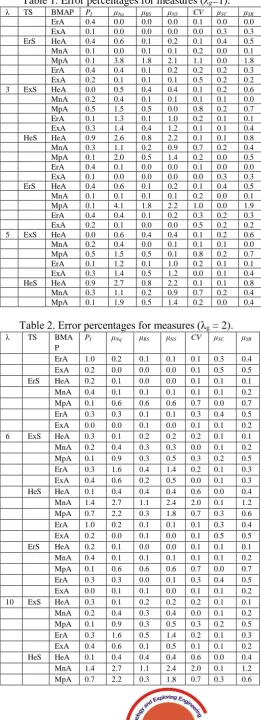
In Tables 1 and 2 the (absolute) error percentage, which is defined as 100 |analytical − simulated|/analytical% is displayed for various scenarios. By looking at the entries in these Tables 1 and 2, we outline a good agreement of the results of numerical simulation and the analytical results reported in [5]. While all the (absolute) error percentages are all very small (none exceeding 5%) with the largest one is 4.1%, a closer look at the analytical and simulated values for this measure (namely, μNq) are, respectively, 2.14795 and
[image:3.595.305.567.57.779.2]2.0601, which are close enough for all practical purposes.
Table 1. Error percentages for measures (
λg
=1).
λ TS BMAP PI μNq μBS μNS CV μSC μSRErA 0.4 0.0 0.0 0.0 0.1 0.0 0.0 ExA 0.1 0.0 0.0 0.0 0.0 0.3 0.3 ErS HeA 0.4 0.6 0.1 0.2 0.1 0.4 0.5 MnA 0.1 0.0 0.1 0.1 0.2 0.0 0.1 MpA 0.1 3.8 1.8 2.1 1.1 0.0 1.8 ErA 0.4 0.4 0.1 0.2 0.2 0.2 0.3 ExA 0.2 0.1 0.1 0.1 0.5 0.2 0.2 3 ExS HeA 0.0 0.5 0.4 0.4 0.1 0.2 0.6 MnA 0.2 0.4 0.1 0.1 0.1 0.1 0.0 MpA 0.5 1.5 0.5 0.0 0.8 0.2 0.7 ErA 0.1 1.3 0.1 1.0 0.2 0.1 0.1 ExA 0.3 1.4 0.4 1.2 0.1 0.1 0.4 HeS HeA 0.9 2.6 0.8 2.2 0.1 0.1 0.8 MnA 0.3 1.1 0.2 0.9 0.7 0.2 0.4 MpA 0.1 2.0 0.5 1.4 0.2 0.0 0.5 ErA 0.4 0.1 0.0 0.0 0.1 0.0 0.0 ExA 0.1 0.0 0.0 0.0 0.0 0.3 0.3 ErS HeA 0.4 0.6 0.1 0.2 0.1 0.4 0.5 MnA 0.1 0.1 0.1 0.1 0.2 0.0 0.1 MpA 0.1 4.1 1.8 2.2 1.0 0.0 1.9 ErA 0.4 0.4 0.1 0.2 0.3 0.2 0.3 ExA 0.2 0.1 0.0 0.0 0.5 0.2 0.2 5 ExS HeA 0.0 0.6 0.4 0.4 0.1 0.2 0.6 MnA 0.2 0.4 0.0 0.1 0.1 0.1 0.0 MpA 0.5 1.5 0.5 0.1 0.8 0.2 0.7 ErA 0.1 1.2 0.1 1.0 0.2 0.1 0.1 ExA 0.3 1.4 0.5 1.2 0.0 0.1 0.4 HeS HeA 0.9 2.7 0.8 2.2 0.1 0.1 0.8 MnA 0.3 1.1 0.2 0.9 0.7 0.2 0.4 MpA 0.1 1.9 0.5 1.4 0.2 0.0 0.4
Table 2. Error percentages for measures (λ
g= 2).
λ TS BMAP
PI μNq μBS μNS CV μSC μSR
IV. ILLUSTRATIVEEXAMPLES
In this section we will discuss a few illustrative examples based on simulated results. In addition to the eight system performance measures listed in Section 2, we will also consider the following measures, one dealing with tail probabilities and the other with the BP. This measure will depend on the batch size distribution and will enable us to see the effect of variation/correlation in the arrival process as well as service time distribution.
9. Probability that the number in the queue exceeds a certain value, P (Nq > n), n ≥ 0.
10. Mean BP, μBP, both partial and full ones, will be considered. Note that it will be clear from the context in the example below whether we are dealing with partial or full BP.
For the arrival processes we consider the same five BMAPs listed in Section 3. Further, we add the following two service time distributions to the ones listed in Section 3, the first, shifted exponential, belonging to the class of so-called log-concave distributions and the second, Weibull, being heavy-tailed. The probability density functions are as follows:
ToS 4: Shifted Exponential (SeS). The density of a SeS with a shift of magnitude 0.2 is given by
𝑓(𝑡) = 1.25𝑒−1.25 (𝑡−0.2), 𝑡 ≥ 0.2.
ToS 5: Weibull (WeS). The 2-parameter Weibull considered here has the probability density function
𝑓(𝑡) = (2𝑡)−0.5𝑒−√2𝑡, 𝑡 ≥ 0.
In our examples below we consider the above five BMAPs (with three batch size distributions as mentioned earlier), five service time distributions, take λg = c, and fix the service rate, μ = 1. Note that by taking λg = c we compare different multi-server queueing systems in such a way that on the average each server has a (group) arrival rate of 1.
A. Example 1
In this example, we vary c = 1, 2, 5, 10, and look at 300 scenarios through five types of arrivals, five services, three batch size distributions, and four values for the number of servers. We study the measures defined above, making one more convention: we define the coefficient of variation of sojourn time in the system as 𝐶𝑉 = 𝜎𝑊𝑠⁄𝜇𝑊𝑠.
[image:4.595.67.272.642.782.2]First, we display in Table 3, the significance (at 5% level) of various measures with regard to the type of arrivals (TaP), the type of services (ToS), the number of servers (c), and the type of batch size distribution (BsD). Here an “X” indicates significance at 5% level and a blank space indicates insignificance at the same level.
Table 3. Significance of measures
Measure c TaP ToS BsD
P (Nq > 1) X X X X
P (Nq> 2) X X X X P (Nq> 4) X X X
P (Nq> 8) X X X P (Nq> 16) X X X
P (Nq> 32) X X
PI X X X
μNq X X
μBS X X X
CV X X X
An examination of the entries of Table 3 indicates the following key observations for the range of the parameter values considered.
1. Batch size distribution plays a significant role in the case of the two tail probabilities, P (Nq > 1)and P (Nq > 2). However, it doesn’t play a significant role in the other measures. The insignificance of the batch size distribution for the system measures (other than the tail probabilities) considered here is proved in [5].
2. For all measures considered here, the type of service times, ToS, and the number of servers (c), play a significant role indicating items such as variability in the service times, heavy tails, concavity, and the number of resources affects the system measures appreciably.
3. In almost all cases, the type of arrival process (TaP) affects significantly the system performance measures. The exceptions appear to be the mean number of customers in the queue and the tail probability, P (Nq > 32).
We did a statistical analysis, including multiple comparisons, on the simulated data with regard to c, TaP, ToS, and BsD and we summarize the key observations below.
1. With regard to P (Nq> 1) and P (Nq> 2), we noticed: a. a decreasing trend as c is increased. This is as is
to be expected since a higher c (in spite of having the same (group) arrival rate of 1 per server) will help to reduce the number of customers waiting in the queue.
b. ErA producing a higher value for these measures; MpA producing the least value (about 25% of the ErA one). The trend of this measure decreasing with increasing variability in the interarrival times (among renewal processes) holds true. c. while HeS and WeS produced two largest values,
ErS yielded the smallest value in the case of both measures.
d. while BsD 3 yielded the largest value, BsD 1 produced the smallest value. This measure for BsD 2 is significantly different from BsD 1 but not from BsD 3.
2. With respect to P (Nq > n), n = 4, 8, 16, 32, we noticed similar (to P (Nq > 1)) observations except that there was no significant difference with respect to the type of distribution used for batch size distribution (BsD). 3. As proved in [5] the measures: PI, μNq, CV, μSC are
insensitive to BsD. In addition to these measures, even the μBPis insensitive to the type of distribution used for the batch size.
4. The measure, PI, is such that
a. it decreases as c increases in all cases, which is as expected and coincides with observations given for P (Nq > 1).
arrivals and the largest is for the MpA arrivals. c. HeS and WeS produce the largest value with
ErS and SeS yielding the smallest. 5. The measure, μNq, is such that
a. it decreases as c increases in all scenarios. b. HeS produces the largest value while ErS
yielding the smallest.
6. When we look at μBS, which stands for the mean number of customers in a service, we notice that this measure
a. decreases as c increases in all scenarios. b. for MpA arrivals, appears to yield the largest
value while ErA producing the smallest one. c. for HeS and WeS arrivals, produce the largest value with the rest, namely, ErS, ExS and SeS yielding the smallest.
7. Finally, we look at the coefficient of variation, CV, of the sojourn time in the system and observe that
a. this increases as c increases in all cases. b. the largest value appears to occur for both
MpA and ErA arrivals, while the smallest one is registered for MnA arrivals.
c. HeS produce the largest value with ErS yielding the smallest.
The purpose of the next example is to compare partial and full BPs. We do so by looking at the mean BP, coefficient of variation of BP, and the ratio of the BP to the corresponding mean sojourn time. Note that the rest of the measures (see above) do not depend on the type of BP.
B. Example 2
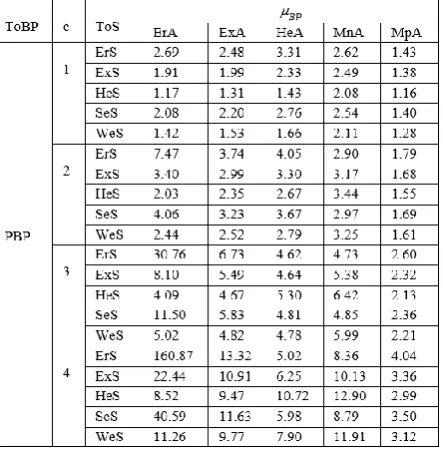
[image:5.595.60.282.528.755.2]This example is similar to Example 1 except that now we vary c = 1, 2, 3, 4 and vary the other parameters as in Example 1. Our main focus here is on the mean BPs (μBP) - both partial (PBP) and full (FBP) - as well as on the ratio of mean BP to the mean sojourn time. In Table 4 (split into many) we display these two measures under various scenarios.
Table 4. Mean BP and its ratio to mean sojourn time
A quick look at the entries in Table 4 reveals the following observations.
μBP > μWsin the case when c = 1for all scenarios. This is mainly due to the fact that all waiting customers at the beginning of a service will be served. It is worth comparing this to the one in the case of classical queues. In [4], it is shown that for a variety of combinations of arrival and services, μBP
> μWs and for some others μBP < μWsfor single as well as multiple-server cases.
2. With regard to PBP, we see μBP > μWs for all scenarios considered here. Again, this is not surprising and agrees with intuition due mainly to providing the type of group services considered here.
3. With regard to FBP, we notice μBP < μWs in all but three scenarios considered here. These three scenarios’ (all corresponding to HeA arrivals) values are not far away from 1 and could be attributed to sampling error. It is worth pointing out that by definition the mean BP under “full” will always be less (unless c = 1 in which case it will be equal) than the corresponding “partial” one, and we see that in our simulated results this inequality also holds.
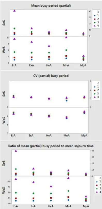
Figure 1. Selected measures under various scenarios for SeS and WeS services
Figure 1. Selected measures under various scenarios for SeS and WeS services
Finally, we compare the two services, SeS and WeS. The plots of selected measures are given in Figure 1. Recall that WeS is a heavy tailed distribution while SeS is log-concave one. A quick look at the plots in Figure 1 reveals the distinct role of heavy tailed services with regard to the (full and partial) mean BPs, coefficient of variation of the (full and partial) BPs, and the ratio of (full and partial) mean BPs to the corresponding mean sojourn time.
V. CONCLUSION
[image:6.595.331.529.51.458.2] [image:6.595.84.288.330.734.2]We also studied the partial and full busy periods, which are important characteristics of a multi-server system. These results might be of practical interest for various fields of application, including the distributed computing systems, wireless transmission systems and solid state drives.
REFERENCES
1. Artalejo J.R., Gomez-Correl A., He Q.M. "Markovian arrivals in stochastic modelling: a survey and some new results" in Statistics and Operations Research Transactions, 2010, 34, 2, pp. 101–144. 2. Chakravarthy S.R. "The batch Markovian arrival process: A review
and future work" in Advances in Probability Theory and Stochastic Processes, Notable Publications Inc., NJ, 2001, pp. 21–39. 3. Chakravarthy S.R. "Markovian arrival processes" in Wiley
Encyclopedia of Operations Research and Management Science, Published Online: 15 JUN 2010, DOI:
10.1002/9780470400531.eorms0499
4. Chakravarthy, S.R. "Busy period analysis of GI/G/c and MAP/G/c queues" in Performance Prediction and Analytics of Fuzzy, Reliability and Queueing Models: Theory and Applications, 2019, pp.1-31. DOI: 10.1007/978-981-13-0857-4_1
5. Chakravarthy, S.R., Shruti, and Rumyantsev, A. "Analysis of a queueing model with batch Markovian arrival process and general distribution for group clearance" Submitted for Publication. 6. Jayaraman, R. and Matis, T. I. "Batch Arrivals and Service Single
Station Queues" in Wiley Encyclopedia of Operations Research and Management Science DOI:10.1002/9780470400531.eorms0095 7. Kelton, W.D., Sadowski, R.P., Swets, N.B. “Simulation with
ARENA” Fifth ed., McGraw-Hill, New York, 2010.
8. Lucantoni D., Meier-Hellstern K.S., and Neuts M.F. “A single-server queue with server vacations and a class of nonrenewal arrival processes” in Advances in Applied Probability, 1990, vol. 22, pp. 676–705, DOI: 10.2307/1427464.
9. Lucantoni D.M. “New results on the single server queue with a batch Markovian arrival process” in Stochastic Models, 1991, vol. 7, pp. 1– 46.
10. Neuts M.F. “A versatile Markovian point process” in Journal of Applied Probability, 1979, vol. 16, pp. 764–779, DOI: 10.1017/S0021900200033465.
11. Neuts M.F. “Matrix-geometric solutions in stochastic models: An algorithmic approach” The Johns Hopkins University Press, Baltimore, MD, 1981.
12. Neuts M.F. “Structured stochastic matrices of M/G/1 type and their applications” Marcel Dekker, NY, 1989.
13. Neuts M.F. “Models based on the Markovian arrival process” in IEICE Transactions on Communications, 1992, E75B, pp. 1255– 1265.
AUTHORSPROFILE
Srinivas R. Chakravarthy received his Ph.D from the University of Delaware, USA. He is now professor of Industrial Engineering & Statistics in the Departments of Industrial and Manufacturing Engineering & the Department of Mathematics, Kettering University, Flint, USA. His research interests include applied stochastic modeling, algorithmic probability, queueing, reliability, inventory, and simulation. He has published more than 110 papers. His professional activities include serving as the Area Editor for the journal, Simulation Modelling Theory and Practice and Advisory Editor for Queueing Models and Service Management.