Robust Flight Control Systems
E. A. Minisci,
1G. Avanzini
2and S. D’Angelo
2 1Department of Aerospace Engineering, University of Glasgow, Glas-gow, G12 8QQ, Scotland
2
Department of Aerospace Engineering, Politecnico di Torino, Turin, 10129, Italy
The aim of this work is to demonstrate the capabilities of evolutionary methods in the design of robust controllers for unstable fighter aircraft in the framework of H∞ control theory. A multi–objective evolutionary algorithm is used to find the controller gains that minimize a weighted combination of the infinite–norm of the sensitivity function (for disturbance attenuation requirements) and complementary sensitivity function (for robust stability requirements). After considering a single operating point for a level flight trim condition of a F-16 fighter aircraft model, two different approaches will then be considered to extend the domain of validity of the control law: 1) the controller is designed for different operating points and gain scheduling is adopted; 2) a single control law is designed for all the considered operating points by multiobjective minimisation. The two approaches will be an-alyzed and compared in terms of efficacy and required human and computational resources.
Keywords Evolutionary optimization, Robust control, Aircraft control
1 Introduction
In this paper a control synthesis technique in the framework of H∞ control theory is
de-veloped, based on the application of a modern multi–objective evolutionary optimization algorithm to the associated minimization problem. In the last two decades, multiple redun-dant, full authority, fail/safe operational, fly–by–wire control systems have been brought to a very mature state. As a result, many aircraft, from earlier designs such as the F-16, F-18, and Tornado through the more recent Mirage 2000, European Fighter Aircraft (EFA), Rafale, and advanced demonstrators such as X-29 and X-31, are highly augmented, actively controlled vehicles that possess either a marginal or negative static stability margin without augmentation, for reasons related to improved performances, weight/cost reduction, and/or low observability.
state. At the same time, modern high performance fighter aircraft are characterized by an extended flight envelope in order to allow the pilot to reach unprecedented maneuvering capabilities at high angles of attack. Such a result can be achieved only if the control system maintains adequate performance in presence of considerable variations of the air-craft response characteristics, avoiding instabilities related to the presence of control surface position and rate saturation limits.
Such a result can be obtained by use of robust controllers. H∞ control theory was
de-veloped in this framework, in order to provide robustness to the closed–loop system to both external disturbance and model uncertainties of known “size”. The controller is synthe-sized by minimizing the infinite norm of the system, determined as the maximum singular value ¯σ of the tranfer function matrix G(s) for a multi–input/multi–output (MIMO) sys-tem, where ¯σ represents the maximum gain for a (disturbance) signal in the exptecred frequency range. The system will be robust to the worst expected disturbance if ¯σ is less than 1, in which case all the disturbances will be attenuated by the closed–loop system. The cost of robustness is a certain degree of “conservativeness” of the controller, which may reduce closed–loop performance. For this reason the requirement for robust stability may be accompanied by requirements in the time domain (such as raise time, overshoot, and settling time). These latter requirements can be enforced as inequality constraints to the optimization problem that must solve the minimization problem while pursuing a minimum acceptable level of performance. These acceptable level can be easily derived in aircraft application from requirements for handling qualities.
The synthesis of the controller will be performed by use of an evolutionary optimi-sation algorithm, motivated by the need for fulfilling different (and possibly competing) requirements in different flight conditions. Highly manoeuvrable aircraft control offers a particularly challenging scenario, where on one side it is unlikely that a single controller synthesized for a given trim operating point performs well over the a sufficiently wide por-tion of the operating envelope, even by use of robust techniques. In this respect, the classic solution is to use gain scheduled controllers, where the gain are varied as a function of ref-erence parameters for the flight condition (e.g. Mach number or dynamic pressure). This classical procedure allows for adapting the system to parameter variation but still requires a certain degree of robustness when the aircraft is flying off–nominal conditions betweem the trim point where the controllers were synthesized. For this reason a gain scheduled controller for an F–16 fighter aircraft reduced short period model will be derived in three different conditions and gain scheduling used for interpolating the gains between the oper-ating points. The F–16 offers a good test–benchmark for the technique as it features most of the characteristics of a modern jet fighter (instability, high-α flight, etc.).
This approach will be compared with the synthesis of a single robust controller derived by enforcing simultaneously the requirements in all the considered operating points. In such a case, a single controller is derived which will be affected by a certain degradation of per-formance in the nominal operating points. But if the off–nominal behaviour is comparable, the advantage of a simpler, scheduling–free controller may be considerable.
After the description of aircraft model and control system architecture and a brief review ofH∞control theory in the next Section, the optimization method used is briefly recalled in
2 Aircraft dynamic model and control system architecture
2.1 Equations of motion and simplifications
The longitudinal equations of motion of a rigid aircraft are expresse by a set of 4 ordinary differential equations in the form
˙
u = −qw−gsinθ+ 0.5ρV2
SCx+T/m
˙
w = qu+gcosθ+ 0.5ρV2
SCz/m (1)
˙
q = 0.5ρV2
ScC¯ m/Iy ; θ˙=q
where the state variables are the velocity componentsuandw(withV2 =u2
+w2
), the pitch angular velocity q and the pitch angleθ. The control variables are the elevetor deflection δE (which acts on the pitch moment aerodynamic coefficient Cm, but it affects the force
coefficients Cx and Cz as well) and the throttle setting δT, suche the thrust delivered by
the engine is T =Tmax(h, M)δT.
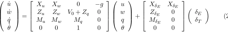
It is possible to linearize the equations of motion in the neighbourhood of a trim condi-tion. By use of a set of stability axes for a level flight condition at velocity V0, one gets a fourth order linear system in the form
˙ u ˙ w ˙ q ˙ θ =
Xu Xw 0 −g
Zu Zw V0+Zq 0
Mu Mw Mq 0
0 0 1 0
u w q θ +
XδE XδE
ZδE 0
MδE 0
0 0 δE δT (2)
The stability derivatives in Eq. 2 depend on the considered flight condition. This means that the response of the aircraft to control action will vary withV0. In order to deal with a simplified model, it is possible to consider the response to a reduced order short period model, under the assumption that attitude variables (q and α ≈w/V0) respond to control input on a faster time–scale then trajectory ones (namely velocityV and flight–path angle γ, where for longitudinal flight it is θ=α+γ), so thatV can be considered approximately constant during an attitude manoeuvre. The reduced order model is given by
˙ α ˙ q =
Zα 1 +Zq/V0 Mα Mq
α q
+
ZδE
MδE
δE (3)
Model fidelity is enhanced by including a simple first order actuator model for the respons of elevator deflection to pilot or automatic control inputs:
˙ δE =
1 τA
(δEcom−δE) (4)
In what follows, an F-16 fighter aircraft model will be considered. The original model, taken from Ref. 1, features a nonlinear aerodynamic model for −10 ≤ α ≤ 45 deg and
|β| ≤30 deg. Finite differences are used to linearize the aircraft model in the neighbourhood of each trim condition and obtain approximate values for the stability derivatives in Eqs. (2) and (3).
[image:3.595.124.509.347.404.2]2.2 Longitudinal Stability and Control augmentation system
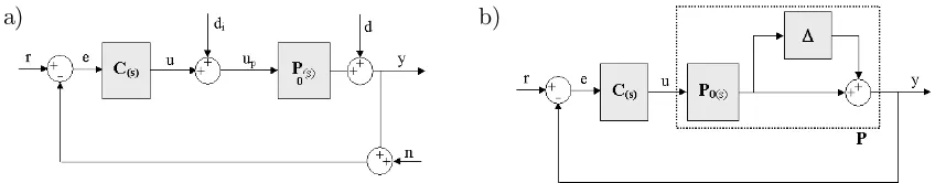
Figure 1: Control system architecture.
artificial static stability (α feedback). In this latter case a filter is included for reducing α sensor noise, with a cut–off frequency of τF = 10 rad/s (that is, F(s) =τF/(s+τF)).
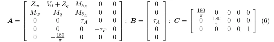
The control augmentation system transforms the longitudinal pilot command into a rate command, where the tracked variable is the pitch angular velocityq. In order to provide the system with zero steady–state error an integrator is included in the pitch angular velocity error channel. The resulting open loop dynamics is described by a linear system of ordinary differential equations in the form
˙
x=Ax+Bu ; y=Cx (5)
where the state vector isx= (α, q, δE, αF, ε)T (whereεis the integrator variable, such that
˙
ε=rq−q), while the only input variable is the pitch velocity reference signalrq. Provided
that the output variables are y = (α, q, ε)T, the state, control, and output matrices are
defined as
A=
Zw V0+Zq MδE 0 0
Mw Mq MδE 0 0
0 0 −τA 0 0
0 0 0 −τF 0
0 −180
π 0 0 0
; B =
0 0 τA
0 0
; C =
180
π 0 0 0 0
0 180
π 0 0 0
0 0 0 0 1
(6)
respectively. The optimization algorithm will be exploited in order to find the gains of the stability augmantation system (Kα andKq) and the integral gain of the control
autmenta-tion system (Ki).
2.3 Robust control
Consider the system depicted in Fig. 2, whereP0(s) is the nominal model of a plant with ni inputs and no outputs, C(s) is the controller, r(s) is the reference input signal y(s), d
is the noise on the output signal and n is the noise on the sensors. Given the definition of the output transfer matrix asLo=P0C, the sensitivity at the output is defined as the transfer matrix y/d, that is
So = (I +Lo)
−1
, y=Sod (7)
and the complementary sensitivity function at the output is
To=I−So=Lo(I+Lo)
−1
a) b)
Figure 2: General feedback configuration (a); feedback configuration with multiplicative uncerntainties of the nominal model (b).
From the system represented in Fig. 2, it is easy to derive that
y=Tor−Ton+SoP di+Sod (9)
It is thus clear that in order to eliminate or at least reduce the effects of noise on the response of the system, it is necessary to operate onTo and So.
Moreover, apart from external noises affecting the signals, the system may be charac-terized by other kind of uncertainties. Usually, the nominal model P0, due to simplifying assumptions and/or linearization, does not correspond to the actual plant. Taking into account a multiplicative uncertainty on the plant model (Fig. ??), brings to the following expression for the output:
y= To+ ∆To
I+ ∆To
r (10)
In order to reduce the effect of the uncertainty it is necessary to tailor the complementary sensitivity function of the uncertainty itself, ∆To.
The main idea behindH∞ control theory and the design process derived in this
frame-work is to find the values of the controller parameters by minimizing appropriately the infinite norm of the weighted sensitivity and complementary sensitivity functions. In order to achieve this result, the following functions need to be minimized:
kW1(s)So(s)k= min ; kW3(s)To(s)k= min (11)
that is, the effect of noises on the output (Eq. 11 and that of uncertainties of the nominal model P0 is reduced.
Since the H∞ norm of a systemG(s) is
kGk∞= sup
ω ¯σ(
G(jω)) (12)
where ¯σ(·) is the maximum singular value, this kind of norm provides the worse gain for a sinuisoidal input for a determined frequency, corresponding to the worse energetic gain of the system. The use of weighted functions allows to deal with different kind of signals, when MIMO systems are considered. Moreover, and more important, weights allow to focus the optimization process only within prescribed frequency ranges. As an example, in order to reduce low frequency noise a weight function with high gains at low frequency will be used, that is, it will be
kWg(s)G(s)k∞<1 ; kG(s)k∞<
1
Wg(s)
(13)
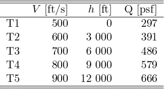
Table 1: Trim conditions
V [ft/s] h [ft] Q [psf] T1 500 0 297 T2 600 3 000 391 T3 700 6 000 486 T4 800 9 000 579 T5 900 12 000 666
Presentatione dell’algoritmo di ottimizzazione
For the first approach, the optimization process is aimed to minimize the function resulting from the sum of the sensitivity and complementary sentitivity function, each appropriately weighted, for three different trim conditions. The optimal gains are then interpolated and tested by means of system linearized for intermediate trim conditions. The objective function is
F =|W1(s)S(s)k∞+|W3(s)T(s)k∞ (14)
where W1 is imposed so that the action on the sensitivity function is enfasized in the low frequency zone, where the main disturbance, which can affect the aircraft performance, belong to, whileW3 is modeled on the basis of assumed uncertainties on the nominal model of the plant. The weight functions are
W1= 1 + 100s
100s+ 1; W3=
100 + 10s
s+ 1000 (15)
Moreover, the constraints on peek time tp, settling time ts and overshoot Mp are set for
each trim condition as follows
tp ≤3[sec]; ts≤4[sec]; Mp≤0.2 (16)
The 3-dimensional search domain is bounded bylb= (−30,−30,−30)T andub= (0,0,0)T.
The second approach provides a three points optimization process, which takes care of the 3 objective functions and the 9 constraints at the same time and, again, a test of the system performance for intermediate trim conditions.
4 Results and discussion
Five trim conditions for the F–16 aircraft model were considered (Tab. 1). Trim condition 1, 3 and 5 (T1, T2, and T3) were considered for controller gain synthesis while conditions 2 and 4 (T2 and T4) were used for simulation of the closed–loop behaviour in off–nominal conditions. Controller 1 (C1) is based upon gain scheduling with respect to dynamic pres-sure, while the second ontroller (C2) employs a fixed set of gains as outlined in the previous section.
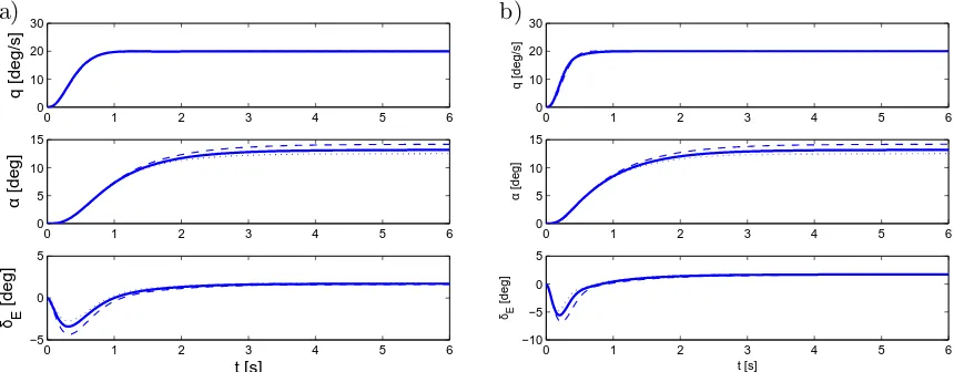
Figure 3 shows the results obtained from a simulation of the closed–loop response to a step input on the input channel rq for C1 (left) and C2 (right) in three different trim
0 1 2 3 4 5 6 0
10 20 30
q [deg/s]
0 1 2 3 4 5 6
0 5 10 15
α
[deg]
0 1 2 3 4 5 6
−5 0 5
δ E
[deg]
t [s]
0 1 2 3 4 5 6
0 10 20 30
q [deg/s]
0 1 2 3 4 5 6
0 5 10 15
α
[deg]
0 1 2 3 4 5 6
−10 −5 0 5
δE
[deg]
t [s]
[image:7.595.84.514.102.270.2]a) b)
Figure 3: Step responses of scheduled (a) and global (b) controllers in T1 (dashed line), T2 (thick line), and T3 (dotted line).
points (T1 and T3), thus proving that both the gain scheduling and the global approaches provides the required degree of robustness with respect to model parameters variations. Note that similar results are also obtained when considering T3 and T5 as reference trim conditions for the controller gain synthesis and T4 as the off–nominal condition, cases not reported in the figures for the sake of conciseness.
Surprisingly enough, the global controller appears to better exploit the available control power in all the considered situations: the response on theq–channel is faster, yet perfectly damped, with no or marginal overshoot, with a faster variation of the control variable,δE,
which, nonetheless remains compatible with saturation and rate–saturation constraints. In this respect, the expected result was that the global synthesis approach should provide a more conservative controller, as a compromise between different operating points.
It is not easy to explain the outcome of the analysis performed. One trivial explanation is that the optimization process for single operating points simply did not succeed in finding a global optimum and was stopped for a locally optimal solution, but it is unlikely that such a situation occurred for all the three considered cases. As a consequence, a more likely explanation is that, in some not yet fully understood way, the optimal control problem for a single operating point penalizes more heavily controllers that may evolve subsequently into more aggressive (optimal) ones.
At the same time, it should be underlined that the global controller appears to be unable to satisfy constraints on robustness to variation of system parameters in the third operating point used for controller synthesis (T5). As a matter of fact, the controller is robust to reasonable variations of system parameters, as demonstrated by the reported simulations. Nonetheless this property is not proved from the mathematical standpoint for one of the considered operating points. Apparently, only by reducing considerably the rise time, it is possible to achieve the desired level of robustness in all the considered operating points, thus significantly affecting overall system performance.
4 Conclusions and future work
In this paper an evolutionary optimization technique was demonstrated as a means for control gain synthesis in the framework ofH∞ control problems. Two different techniques
operating points, by use of gain scheduling for checking control performance in off–nominal conditions. In the second framework, a single set of gains was searched for, which satisfies control constraints and performance in the same set of operating points. Satisfactory results were obtained in both cases, although the second one provided a more aggressive controller on one side, at the expenses of some lack of robustness.
The research will now focus on improving the search of an optimal solution for both techniques (more aggressive controllers in the first case, robust in the whole considered flight envelope for second one). Moreover, a more demanding scenario will also be considered, where simulations are performed by using the fully nonlinear six-degrees-of-freedom model, in order to assess more convincingly the robustness of the control system to both parameter variations and unmodeled dynamics.
Acknowledgements
Giulio Avanzini is grateful to the Department of Aerospace Engineering of the University of Glasgow for inviting him as visiting lecturer in the Fall semester of Academic Year 2007–08. A grant from the Erasmus Office of the Italian National Agency LLP (Lifelong Learning Program) and support from Politecnico di Torino in the framework of “Young Researchers Program” 2007 are also acknowledged.
References
1. Stevens, B.L., and Lewis, F.L.,Aircraft Control and Simulation, Wiley, New York, 1992 2. Referenza 2