R. Mittleman,8O. Miyakawa,1S. Mohanty,30G. Moreno,9K. Mossavi,2C. MowLowry,5A. Moylan,5D. Mudge,18G. Mueller,24 H. Mu¨ ller-Ebhardt,2S. Mukherjee,30J. Munch,18P. Murray,10E. Myers,9J. Myers,9G. Newton,10K. Numata,20
B. O’Reilly,15R. O’Shaughnessy,12 D. J. Ottaway,8H. Overmier,15B. J. Owen,28Y. Pan,25M. A. Papa,7,3 V. Parameshwaraiah,9M. Pedraza,1S. Penn,39M. Pitkin,10 M. V. Plissi,10R. Prix,7V. Quetschke,24F. Raab,9
D. Rabeling,5H. Radkins,9R. Rahkola,17M. Rakhmanov,28K. Rawlins,8S. Ray-Majumder,3V. Re,6 H. Rehbein,2S. Reid,10D. H. Reitze,24L. Ribichini,2R. Riesen,15K. Riles,21B. Rivera,9D. I. Robertson,10
N. A. Robertson,13,10C. Robinson,23S. Roddy,15 A. Rodriguez,4A. M. Rogan,16J. Rollins,36 J. D. Romano,23J. Romie,15 R. Route,13S. Rowan,10A. Ru¨ diger,2L. Ruet,8P. Russell,1K. Ryan,9
S. Sakata,37M. Samidi,1L. Sancho de la Jordana,40 V. Sandberg,9V. Sannibale,1S. Saraf,13 P. Sarin,8B. S. Sathyaprakash,23S. Sato,37P. R. Saulson,26R. Savage,9S. Schediwy,11R. Schilling,2
R. Schnabel,2R. Schofield,17 B. F. Schutz,7,23P. Schwinberg,9S. M. Scott,5S. E. Seader,16 A. C. Searle,5B. Sears,1F. Seifert,2D. Sellers,15A. S. Sengupta,23P. Shawhan,1B. Sheard,5
D. H. Shoemaker,8A. Sibley,15 X. Siemens,3D. Sigg,9A. M. Sintes,40,7B. Slagmolen,5 J. Slutsky,4J. Smith,2M. R. Smith,1P. Sneddon,10 K. Somiya,2,7C. Speake,6O. Spjeld,15
K. A. Strain,10D. M. Strom,17A. Stuver,28 T. Summerscales,28K. Sun,13 M. Sung,4 P. J. Sutton,1D. B. Tanner,24M. Tarallo,1R. Taylor,1R. Taylor,10J. Thacker,15
K. A. Thorne,28K. S. Thorne,25 A. Thu¨ ring,27K. V. Tokmakov,14C. Torres,30 C. Torrie,1G. Traylor,15M. Trias,40W. Tyler,1D. Ugolini,41C. Ungarelli,6 H. Vahlbruch,27 M. Vallisneri,25M. Varvella,1S. Vass,1A. Vecchio,6J. Veitch,10
P. Veitch,18S. Vigeland,22A. Villar,1C. Vorvick,9S. P. Vyachanin,14 S. J. Waldman,1L. Wallace,1H. Ward,10R. Ward,1K. Watts,15D. Webber,1
A. Weidner,2A. Weinstein,1R. Weiss,8S. Wen,4K. Wette,5J. T. Whelan,38,7 D. M. Whitbeck,28S. E. Whitcomb,1B. F. Whiting,24C. Wilkinson,9 P. A. Willems,1B. Willke,27,2I. Wilmut,34W. Winkler,2C. C. Wipf,8
S. Wise,24A. G. Wiseman,3G. Woan,10 D. Woods,3R. Wooley,15 J. Worden,9W. Wu,24I. Yakushin,15 H. Yamamoto,1Z. Yan,11
S. Yoshida,42N. Yunes,28M. Zanolin,8L. Zhang,1C. Zhao,11 N. Zotov,43 M. Zucker,15H. zur Mu¨ hlen,27and J. Zweizig1
( The LIGO Scientific Collaboration)44 Received 2006 September 21; accepted 2006 November 30
ABSTRACT
The Laser Interferometer Gravitational-Wave Observatory ( LIGO) has performed the fourth science run, S4, with significantly improved interferometer sensitivities with respect to previous runs. Using data acquired during this science run, we place a limit on the amplitude of a stochastic background of gravitational waves. For a frequency in-dependent spectrum, the new Bayesian 90% upper limit isGW; H0/ 72 km s1 Mpc1
2<6:5;105. This
is currently the most sensitive result in the frequency range 51Y150 Hz, with a factor of 13 improvement over the previous LIGO result. We discuss the complementarity of the new result with other constraints on a stochastic background of gravitational waves, and we investigate implications of the new result for different models of this background.
Subject headingg:gravitational waves
1. INTRODUCTION
A stochastic background of gravitational waves (GWs) is ex-pected to arise as a superposition of a large number of unresolved sources, from different directions in the sky and with different polarizations. It is usually described in terms of the GW spectrum,
GW(f)¼
f
c
dGW
df ; ð1Þ
where dGW is the energy density of gravitational radiation contained in the frequency range ftof þdf(Allen & Romano
1999),c is the critical energy density of the universe, and f is frequency (for an alternative and equivalent definition of GW(f) see, e.g., Baskaran et al. [2006]; Grishchuk et al. [2006]).
Many possible sources of stochastic GW background have been proposed, and several experiments have searched for it (see Maggiore 2000; Allen 1997 for reviews). Some of the proposed theoretical models are cosmological in nature, such as the amplifi-cation of quantum vacuum fluctuations during inflation (Grishchuk 1975, 1997; Starobinsky 1979), preYbig bang models (Gasperini & Veneziano 1993, 2003; Buonanno et al. 1997), phase transitions ( Kosowsky et al. 1992; Apreda et al. 2002), and cosmic strings (Caldwell & Allen 1992; Damour & Vilenkin 2000, Damour & Vilenkin 2005). Others are astrophysical in nature, such as rotating neutron stars ( Regimbau & de Freitas Pacheco 2001), supernovae (Coward et al. 2002), or low-mass X-ray binaries (Cooray 2004).
While some of these models predict complex GW spectra, most of them can be well approximated with power laws in the
39
Hobart and William Smith Colleges, Geneva, NY.
40 Universitat de les Illes Balears, Palma de Mallorca, Spain. 41
Trinity University, San Antonio, TX.
42 Southeastern Louisiana University, Hammond, LA. 43
Louisiana Tech University, Ruston, LA.
Laser Interferometer Gravitational-Wave Observatory ( LIGO) frequency band. Hence, we focus on power-law GW spectra:
GW(f)¼
f
100 Hz
!
; ð2Þ
where is the amplitude corresponding to the spectral in-dex. In particular,0denotes the amplitude of the frequency-independent GW spectrum. We consider the range3< <3. A number of experiments have been used to constrain the spectrum of GW background at different frequencies. Currently, the most stringent constraints arise from large-angle correlations in the cosmic microwave background (CMB; Allen & Koranda 1994; Turner 1997), from the arrival times of millisecond pulsar signals (Jenet et al. 2006), from Doppler tracking of theCassini
spacecraft (Armstrong et al. 2003), and from resonant bar GW detectors, such as Explorer and Nautilus (Astone et al. 1999). An indirect bound can be placed on the total energy carried by gravi-tational waves at the time of the big bang nucleosynthesis (BBN ) using the BBN model and observations ( Kolb & Turner 1990; Maggiore 2000; Allen 1997). Similarly, Smith et al. (2006b) used the CMB and matter spectra to constrain the total energy density of gravitational waves at the time of photon decoupling.
Ground-based interferometer networks can directly measure the GW strain spectrum in the frequency band 10 Hz to a few kHz by searching for correlated signal beneath uncorrelated detector noise. LIGO has built three power-recycled Michelson interfer-ometers, with a Fabry-Perot cavity in each orthogonal arm. They are located at two sites: Hanford, Washington, and Livingston Parish, Louisiana. There are two collocated interferometers at the Washington site: H1, with 4 km long arms, and H2, with 2 km arms. The Louisiana site contains L1, a 4 km interferometer, sim-ilar in design to H1. The detector configuration and performance during LIGO’s first science run (S1) was described in Abbott et al. (2004a). The data acquired during that run were used to place an upper limit of0<44:4 on the amplitude of a frequency independent GW spectrum, in the frequency band 40Y314 Hz (Abbott et al. 2004b). For this limit, as well as in the rest of this paper, we assume the present value of the Hubble parameterH0¼ 72 km s1 Mpc1( Bennet et al. 2003), i.e., when writing 0, we implicitly mean0; H0/ 72 km s1 Mpc1
2
. The most recent bound on the amplitude of the frequency-independent GW spectrum from LIGO is based on the science run S3;0< 8:4;104 for a frequency-independent spectrum in the 69Y 156 Hz band (Abbott et al. 2005).
In this paper, we report much-improved limits on the stochas-tic GW background around 100 Hz, using the data acquired during the LIGO science run S4, which took place between 2005 February 22 and March 23. The sensitivity of the interferometers during S4, shown in Figure 1, was significantly better than S3 ( by a factor 10 at certain frequencies), which leads to an order-of-magnitude improvement in the upper limit on the amplitude of the stochastic GW background:0<6:5;105for a frequency-independent spectrum over the 51Y150 Hz band.
This limit is beginning to probe some models of the stochastic GW background. As examples, we investigate the implications of this limit for cosmic strings models and for preYbig bang models of the stochastic gravitational radiation. In both cases, the new LIGO result excludes parts of the parameter space of these models. The organization of this paper is as follows. Inx2 we review the analysis procedure and present the results inx3. Inx4, we discuss some of the implications of our results for models of a stochastic GW background, as well as the complementarity
be-tween LIGO and other experimental constraints on a stochastic GW background. We conclude with future prospects inx5.
2. ANALYSIS
2.1.Cross-Correlation Method
The cross-correlation method for searching for a stochastic GW background with pairs of ground-based interferometers is described in Allen & Romano (1999). We define the following cross-correlation estimator:
Y ¼ Z þ1
0
df Y(f)
¼ Z þ1
1 df
Z þ1
1
df0T(f f0) ˜s1(f)s˜2(f0) ˜Q(f0); ð3Þ
whereTis a finite-time approximation to the Dirac delta func-tion, ˜s1and ˜s2are the Fourier transforms of the strain time series of two interferometers, and ˜Qis a filter function. Assuming that the detector noise is Gaussian, stationary, uncorrelated between the two interferometers, and much larger than the GW signal, the variance of the estimatorYis given by
Y2 ¼ Z þ1
0
dfY2(f)
T
2
Z þ1
0
d f P1(f)P2(f) ˜Q fð Þ2; ð4Þ
wherePi(f) are the one-sided power spectral densities ( PSDs) of the two interferometers, andTis the measurement time. Op-timization of the signal-to-noise ratio leads to the following form of the optimal filter (Allen & Romano 1999):
˜
Q(f)¼N (f)SGW(f)
P1(f)P2(f); ð5Þ
Fig. 1.— Typical strain amplitude spectra of LIGO interferometers during
where
SGW(f)¼ 3H2
0 102
GW(f)
f3 ; ð6Þ
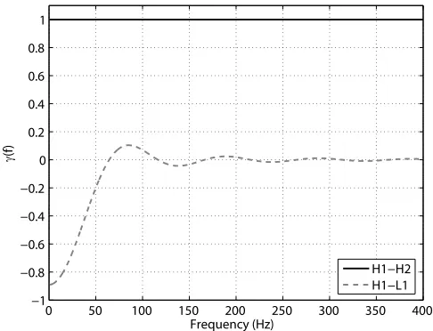
and(f) is the overlap reduction function arising from the dif-ferent locations and orientations of the two interferometers. As shown in Figure 2, the identical antenna patterns of the collo-cated Hanford interferometers imply(f)¼1. For the Hanford-Livingston pair the overlap reduction is significant above 50 Hz. In equations (5) and (6),SGW(f) is the strain power spectrum of the stochastic GW background to be searched. Assuming a power-law template GW spectrum with index(see eq. [2]), the normal-ization constantNin equation (5) is chosen such thath i ¼Y T. In order to deal with data nonstationarity, and for purposes of computational feasibility, the data for an interferometer pair are divided into many intervals of equal duration, andYIandYI
are calculated for each intervalI. The data in each interval are decimated from 16,384 to 1024 Hz and high-pass filtered with a 40 Hz cutoff. As we discuss below, most of the sensitivity of this search lies below 300 Hz, safely below the Nyquist frequency of 512 Hz. The intervals are also Hann windowed to avoid spectral leakage from strong lines present in the data. Since Hann win-dowing effectively reduces the interval length by 50%, the data intervals are overlapped by 50% to recover the original signal-to-noise ratio. The effects of windowing are taken into account as discussed in Abbott et al. (2004b).
The PSDs for each interval [needed for the calculation of
QI(f) and ofYI] are calculated using the two neighboring
inter-vals. This approach avoids a bias that would otherwise exist due to a nonzero covariance between the cross-powerY(f) and the power spectra estimated from the same data ( Bendat & Piersol 2000). It also allows for a stationarity cut, which we describe in more detail below.
We consider two interval durations and frequency resolutions:
1. 60 s duration with 1/4 Hz resolution.—The PSDs are calculated by averaging 58 50% overlapping periodograms ( based on the two neighboring 60 s intervals) in Welch’s mod-ified periodogram method.
2. 192 s duration with1/32 Hzresolution.—The PSDs are calculated by averaging 22 50% overlapping periodograms (based
on the two neighboring 192 s intervals) in Welch’s modified periodogram method.
As we discuss below, the 60 s intervals allow better sensitivity to noise transients and are better suited for data-stationarity cuts. We used this interval duration in the blind analysis. However, after unblinding we discovered a comb of correlated sharp 1 Hz harmonic lines between interferometers. To remove these sharp lines from our analysis without significantly affecting the sen-sitivity, we performed the second analysis with 192 s intervals. The 192 s intervals allow higher frequency resolution of the power and cross-power spectra and are better suited for removing sharp lines from the analysis.
The data for a given intervalIare Fourier transformed (with frequency resolution 1/60 or 1/192 Hz) and rebinned to the fre-quency resolution of the PSDs and of the optimal filter (1/4 or 1/32 Hz, respectively) to complete the calculation ofYI(eq. [3]). Both the PSDs and the Fourier transforms of the data are cal-ibrated using interferometer response functions, determined for every minute of data using a measurement of the interferom-eter response to a sinusoidal calibration force. To maximize the signal-to-noise ratio, the intervals are combined by performing a weighted average (with weights 1/Y2I), properly accounting
for the 50% overlapping as discussed in Lazzarini & Romano (2004).
2.2.Identification of Correlated Instrumental Lines
The results of this paper are based on the Hanford-Livingston interferometer pairs, for which the broadband instrumental cor-relations are minimized. Nevertheless, it is still necessary to in-vestigate whether there are any remaining periodic instrumental correlations. We do this by calculating the coherence over the whole S4 run. The coherence is defined as
(f)¼ jP12(f)j
2
P1(f)P2(f): ð7Þ
The numerator is the square of the cross-spectral density (CSD) between the two interferometers, and the denominator contains the two power spectral densities ( PSDs). We average the CSD and the PSDs over the whole run at two different resolutions: 1 and 100 mHz. Figure 3 shows the results of this calculation for the H1-L1 pair and for the H2-L1 pair.
At 1 mHz resolution, a forest of sharp 1 Hz harmonic lines can be observed. These lines were likely caused by the sharp ramp of a one-pulse-per-second signal, injected into the data ac-quisition system to synchronize it with the Global Positioning System (GPS) time reference. Since the coupling of this signal to the gravitational-wave channel of H1 was much stronger than that of H2, the forest of 1 Hz harmonics is much clearer in the H1-L1 coherence. After the S4 run ended, the sharp ramp signal was replaced by smooth sinusoidal signals, with the goal of sig-nificantly reducing the 1 Hz harmonic lines in future LIGO data runs. In addition to the 1 Hz lines, the 1 mHz coherence plots in Figure 3 also include some of the simulated pulsar lines, which were injected into the differential-arm servo of the interferom-eters by physically moving the mirrors. Both the 1 Hz harmonics and the simulated pulsar lines can be removed in the final anal-ysis, and we discuss this further inx3. Figure 4 shows that the histogram of the coherence at 1 mHz resolution follows the ex-pected exponential distribution, if one ignores the 1 Hz harmonics and the simulated pulsar lines.
[image:3.612.49.292.64.250.2]2.3.Data Quality Cuts
In our analysis, we include time periods during which both interferometers are in low-noise, science mode. We exclude:
1. Time periods when digitizer signals saturate.
2. 30 s intervals prior to each ‘‘lock loss’’; interferometers become increasingly unstable during these intervals, usually due to some external disturbance, until they eventually fail to maintain the fixed distances between mirrors.
We then proceed to calculateYIandYI for each intervalIand
define three data quality cuts. First, we reject intervals known to contain large glitches in one interferometer. These intervals were identified by searching for discontinuities in the PSD trends over the whole S4 run. Second, we reject intervals for whichYI is
anomalously large. This cut is designed to reject intervals that happen during particularly noisy periods, by rejecting about 2% of the intervals in the high-end tail of theYIdistribution. In
par-ticular, for the 192 s analysis, we requireYI<1 s for the H1-L1
pair, andYI <2 s for the H2-L1 pair (recall thatYis normalized
such thath i ¼Y T, withT ¼192 s in this case). The glitch cut and the largecut largely overlap and are designed to remove
particularly noisy time periods from the analysis. Note also that due to the weighting with 1/2
YI, the contribution of these
inter-vals to the final result would be suppressed, but we reject them from the analysis nevertheless. Third, we reject the intervals for which ¼ jYI
0
YIj/YI> . Here,YI is calculated using
the two intervals neighboring intervalI, andY0I is calculated
us-ing the intervalIitself. The optimization of threshold is dis-cussed below. The goal of this cut is to capture noise transients in the data and reject them from the analysis. Figure 5 shows the impact of these cuts for the H1-L1 pair, analyzed with 192 s seg-ments, 1/32 Hz resolution, and with ¼0:3. This figure also shows daily variation in the sensitivity to stochastic GW back-ground, arising from the variation in the strain sensitivity of the interferometers, which is typically worse during the weekdays than during the weekends or nights.
Figure 6 shows the distribution of the residuals for the same analysis. For a given intervalI, the residual is defined as
YI h iY
YI
; ð8Þ
Fig.4.— Histogram of the coherence for H1-L1 (top) and H2-L1 (bottom) at
1 mHz resolution. The histogram follows the expected exponential distribution, with exponent coefficientNavg(the number of time periods over which the
av-erage is made), when the 1 Hz harmonics are removed (‘‘after notching’’). The gray histograms (‘‘before notching’’) show the outliers from the exponential dis-tribution due to the 1 Hz harmonics.
Fig.3.— Coherence calculated for the H1-L1 pair (top) and for the H2-L1 pair
(bottom) over all of S4 data for 1 and 100 mHz resolution. The horizontal dashed lines indicate 1/Navg, the expected level of coherence after averaging overNavg
[image:4.612.43.286.66.460.2] [image:4.612.321.562.69.458.2]whereh iY is calculated using only the data that pass all the data quality cuts. Also note that the data quality cuts remove outliers from the residual distribution, hence making the data more sta-tionary. After the cuts, the Kolmogorov-Smirnov test indicates that the residual distribution is consistent with a Gaussian, for both H1-L1 and H2-L1 analyses with 192 s intervals, 1/32 Hz reso-lution, and¼0:3.
3. RESULTS
3.1.New Upper Limit
We performed a ‘‘blind’’ analysis for the H1-L1 and the H2-L1 pairs with 60 s intervals, 1/4 Hz resolution, and¼0:2. To avoid biasing the results, all data quality cuts were defined based on studies done with a 0.1 s time shift between the two in-terferometers in a pair. Such a time shift removes any GW cor-relations, without significantly affecting the instrumental noise performance. After the data quality cuts were finalized, we made one last pass through the data, with zero time shift, and obtained the final results of the blind analysis.
The results from the blind analysis for the frequency-independent template spectrum ( ¼0) are listed in the first row of Table 1 for H1-L1 and in the first row of Table 2 for H2-L1. These re-sults show no evidence of a stochastic GW background. After com-pleting the blind analysis, we discovered that the instrumental 1 Hz harmonic lines, discussed inx2.2, are correlated between the two sites. We felt compelled on scientific grounds not to ignore these correlations, even though they had been discovered after our ini-tial, blind, analysis was complete.
In order to remove from our results any possible influence of the correlated lines, we repeated our analysis with refined fre-quency resolution of 1/32 Hz. We increased the interval length from 60 to 192 s, which implies that the PSDs are estimated by averaging 22 50% overlapping periodograms. These changes al-lowed us to exclude the 1 Hz harmonics from the analysis while losing only3% of the bandwidth. Besides the low cost in band-width, the advantages of this approach are its simplicity and the fact that it does not introduce new systematics effects. The draw-back, however, was that the 192 s analysis was less able to iden-tify and exclude the noise transients than the 60 s analysis, as shown in Figure 7. As a result, thecut was retuned for the
192 s analysis after the 60 s analysis with zero time shift was completed.
We examined several methods of defining the data quality cuts for the 192 s analysis. First, we calculated thecut in the 60 s analysis with¼0:2 (along with largeand glitch cuts), and then declared 192 s intervals ‘‘bad’’ if they overlapped with the ‘‘bad’’ 60 s intervals. This approach has the advantage that the 60 s analysis is more sensitive to transients, and the disadvantage that a significant fraction of the data is rejected. The results of this approach are summarized in the second row of Tables 1 and 2. Second, we defined all cuts directly on 192 s intervals. We varied the value of(0.2, 0.3, and 0.4) and selected¼0:3 as the op-timal parameter choice. This choice represents the best com-promise between data loss and data quality; it rejects the least amount of data, while still excluding all residual outliers and preserving the Gaussianity of the data. The last three rows of Tables 1 and 2 summarize the results for the three values of. The 192 s analysis was not performed blindly. However, it agrees with our blind 60 s analysis very well, because the con-tribution of the correlated 1 Hz harmonic lines is only about 1.5. It is also more conservative than the blind analysis, since the value of the theoretical error is larger due to a smaller amount of data available in the form of acceptable 192 s intervals (as compared to the 60 s intervals). It also properly handles the known instru-mental correlations at 1 Hz harmonics. Hence, in the remaining part of the paper we focus on the 192 s analysis with¼0:3. For the H1-L1 pair, 12,637 50% overlapping 192 s intervals pass all data quality cuts of this analysis, amounting to 353.9 hr of ex-posure. For the H2-L1 pair, 11,849 intervals pass all data quality cuts of this analysis, amounting to 332.7 hr of exposure.
Figures 8 and 9 show the results of the 192 s analysis with
¼0:3 for H1-L1 and H2-L1, respectively. The top plots in these two figures show the cumulative estimates for the frequency-independent GW template ( ¼0) as a function of time. They indicate that there is no particular time during the run that domi-nates the result. Moreover, the1.65 bounds converge as
1/pffiffiffiffiT, as expected. The middle plots of the two figures show the cross-correlation spectra (i.e., the integrand of eq. [3]). They indicate that there is no particular frequency that dominates the result.
Fig.6.— Distribution of residuals for the H1-L1 pair with 192 s segments. All
data are shown in gray, data that pass data quality cuts are shown in black, and the Gaussian fit to the black histogram is shown as a dashed curve.
Fig.5.—Trend ofY
Iover the whole S4 run for the 192 s intervals of H1-L1
We perform a weighted average of the H1-L1 and H2-L1 re-sults at each frequency bin (with inverse variances as weights). The resulting cross-correlation spectrum and the theoretical error are shown in Figure 10. The frequency range 51Y150 Hz con-tributes 99% of the full sensitivity, as determined by the inverse combined variance. Integrating over this frequency range, we ob-tain the final estimate for the frequency-independent spectrum: 0¼(0:84:3);105.
The dominant systematic uncertainty of this result comes from the amplitude calibration uncertainty of the interferometers. This uncertainty is estimated to be 5% ( L1) and 8% ( H1 and H2), and it is frequency-independent. The uncertainty in the phase of the interferometer strain response is negligible compared to the mag-nitude and statistical uncertainties. Similarly, the effect of timing errors, measured to beP4s, is negligible. Using hardware in-jections, we estimate that the effect of the timing errors on our point estimate isP0.2%.
We then construct the Bayesian posterior distribution for0 using the above estimate, following Loredo (1990). We assume a Gaussian distribution for the amplitude calibration uncertainty [with mean 1 and standard deviation 0ð :052þ0:082Þ1/2
¼0:093], and we marginalize over it. We assume the prior distribution for 0to be the posterior distribution obtained in our previous anal-ysis of the S3 data (Abbott et al. 2005). The 90% upper limit is the value of0for which 90% of the posterior distribution lies be-tween 0 and the upper limit. This procedure yields the Bayesian
90% upper limit ( UL) on0of 6:5;105. This is an improve-ment by a factor 13 over the previous result in the same fre-quency band, established based on the science run S3 (Abbott et al. 2005). To investigate robustness of our result under dif-ferent priors, we repeated the calculation using flat priors for the amplitude calibration uncertainties and using a flat prior for0between 0 and 8:4;104( previous 90% UL by LIGO; Abbott et al. 2005). We found that these different choices of priors have less than 3% effect on the 90% upper limit.
Once the estimate is made for the frequency-independent spec-trum, one can perform appropriate frequency-dependent scal-ings ofY(f) andY(f), recalculate the posterior distributions, and remarginalize to obtain upper limits for other templates, such as the power-law templates with different spectral indices(see eq. [2]). Figure 11 shows the 90% UL as a function of the spec-tral indexobtained for this analysis. Similar results for the S3 run of LIGO, as well as the expected sensitivities of H1-L1 and H1-H2 pairs assuming 1 yr of exposure and design interferom-eter sensitivities, are also shown. The frequency range of interest is defined to include 99% of the full sensitivity, as determined by the inverse variance. For the S4 result, the frequency range varies between 50Y107 Hz for ¼ 3 and 73Y288 Hz for ¼ þ3, as shown in the bottom plot of Figure 11. Note that the ex-pected sensitivity of the collocated Hanford interferometer pair ( H1-H2) is significantly better than that of the H1-L1 pair due to the better antenna pattern overlap (see Fig. 2). However, this
TABLE2
H2-L1 Results
Analysis (1)
(2)
Fraction of Data Excluded (%)
(3)
0(;105) Before Notching
50Y500 Hz (4)
0(;105) After Notching
51Y150 Hz (5)
90% UL (;105)
(6) 60 s ( blind) ... 0.2 4.1 8.210.6 . . . 13.0 192 s... conversion 10.7 3.911.9 7.212.1 16.1 192 s... 0.2 6.1 1.711.6 4.211.8 17.1 192 s... 0.3 4.6 0.611.5 3.311.7 17.5 192 s... 0.4 3.8 3.111.5 6.111.7 15.9
Notes.—H2-L1 results, forH0¼72 km s1Mpc1and for a frequency-independent template spectrum (¼0). Cols. (1) and (2) define the analysis (interval
du-ration andcut). For the 192 s analysis withdenoted as ‘‘conversion’’ (second row), thecut was defined using the 60 s analysis listed in the first row: the 192 s segments are declared ‘‘bad’’ if they overlap with a ‘‘bad’’ 60 s segment. Col. (3): Fraction of the data lost to data quality cuts. Col. (4): Estimates of0for the 50Y500 Hz
range before notching the 1 Hz harmonics and the simulated pulsar lines. Col. (5): Estimates of0for the 51Y150 Hz range after notching the 1 Hz harmonics and the
simulated pulsar lines; this frequency range was determined to be optimal for the combined H1-L1+H2-L1 analysis (see text). Col. (6): The 90% upper limit based on the result in col. (5). For all analyses presented here, the distribution of the residual outliers was consistent with a Gaussian distribution (the Kolmogorov-Smirnov test statistic for comparing the two distributions was greater than 52% in all cases).
TABLE1
H1-L1 Results
Analysis (1)
(2)
Fraction of Data Excluded (%)
(3)
0(;105) Before Notching
50Y500 Hz (4)
0(;105) After Notching
51Y150 Hz (5)
90% UL (;105)
(6) 60 s ( blind) ... 0.2 7.1 6.44.3 . . . 13.0 192 s... conversion 21.0 3.44.9 2.45.0 7.0 192 s... 0.2 10.9 6.14.7 0.14.8 8.0 192 s... 0.3 6.5 4.84.6 0.74.7 7.3 192 s... 0.4 5.0 4.84.6 0.74.7 7.3
Notes.—H1-L1 results, forH0¼72 km s1Mpc1and for a frequency-independent template spectrum (¼0). Cols. (1) and (2) define the analysis (interval
duration andcut). For the 192 s analysis withdenoted as ‘‘conversion’’ (second row), thecut was defined using the 60 s analysis listed in the first row: the 192 s segments are declared ‘‘bad’’ if they overlap with a ‘‘bad’’ 60 s segment. Col. (3): Fraction of the data lost to data quality cuts. Col. (4): Estimates of0for the 50Y500 Hz
range before notching the 1 Hz harmonics and the simulated pulsar lines. Col. (5): Estimates of0for the 51Y150 Hz range after notching the 1 Hz harmonics and the
pair is also more susceptible to instrumentally correlated noise. New analysis methods are being pursued to estimate and sup-press these instrumental correlations ( Fotopoulos 2006).
3.2.Signal Injections
We exercise the analysis procedure described above using simulated stochastic signals injected into the data both in
soft-ware and in hardsoft-ware (see Bose et al. 2003). In particular, we verify that the recovery of the injected signals is not affected by the data quality cuts we impose. The hardware injections are performed by physically moving the mirrors to simulate a sto-chastic GW signal. Three hardware injections were performed during the S4 run, all using a frequency-independent GW spec-trum ( ¼0). Table 3 summarizes the recovery of all of the hard-ware injections. Figure 12 shows the cross-correlation spectrum
Fig.7.—Trend ofYfor the 60 s analysis (gray) and 192 s analysis (black)
over a short period of time. The two bands were scaled to overlap. Note that the gray band is wider, indicating that the 60 s analysis is more sensitive to noise variations.
Fig.8.—H1-L1, 192 s analysis with¼0:3.Top: Cumulative estimate of0
is shown as a function of time.Middle: Cross-correlation spectrumY(f).Bottom: Theoretical uncertaintyY(f) as a function of frequency.
Fig.9.—H2-L1, 192 s analysis with¼0:3.Top: Cumulative estimate of0
is shown as a function of time.Middle: Cross-correlation spectrumY(f).Bottom: Theoretical uncertaintyY(f) as a function of frequency.
Fig.10.— Combined H1-L1+H2-L1 result, 192 s analysis with¼0:3.Top:
for injection 3. It also shows the inverse Fourier transform of the spectrum, which is equivalent to the estimate of0for different values of time lag between two interferometers (for short time lags).
We performed a sequence of software injections, where the injected signal is simply added to the interferometer data in the analysis. We performed 10 trials for 4 injection amplitudes using
about 1/3 of the S4 H1-L1 data. Figure 13 shows that the signal is successfully recovered down to 1;104 in0. Moreover, the theoretical error bars agree well with the standard deviation over the 10 trials. All injections were performed assuming a frequency-independent GW spectrum (¼0).
4. IMPLICATIONS
In this section, we investigate the implications of the new upper limit for some of the models of the stochastic GW background. We also discuss the complementarity of our result with various other experimental constraints on the stochastic GW background.
4.1.Complementarity with Other Measurements and Obser
v
ationsFigure 14 compares different experiments and some of the theoretical models. We note again our assumption regarding
TABLE3
Summary of the Hardware Injection Amplitudes During S4
Injection (1)
H1-L1 Expected (;102)
(2)
H1-L1 Recovered (;102)
(3)
H2-L1 Expected (;102)
(4)
H2-L1 Recovered (;102)
(5) 1... 9.1 7.90.20.8 7.9 6.90.40.6 2... 2.5 2.50.40.2 2.3 1.50.60.2 3... 1.1 0.950.040.10 . . . .
Notes.—Cols. (2) and (4) indicate the expected injection amplitudes for H1-L1 and H2-L1, respectively, based on the signal
in-jected into the differential-arm servo. Cols. (3) and (5) list the recovered values using the H1-L1 and H2-L1 pairs respectively. The recovered values are listed with statistical errors (as defined in eq. [4]) and with systematic errors (estimated using 5% calibration uncertainty in L1 and 8% calibration uncertainty in H1 and H2, added in quadrature). For injection 3, the data of H2 interferometer were compromised due to a failure of the interferometer’s laser.
Fig.11.—Top: 90% UL onas a function offor S3 L1 and S4
L1+H2-L1 combined and expected final sensitivities of LIGO L1 and H1-H2 pairs, assuming LIGO design sensitivity and 1 yr of exposure.Bottom: Frequency band containing 99% of the full sensitivity (as determined by the inverse variance) is plotted as a function offor the S4 result.
Fig.12.— H1-L1 injection 3 (with intended injection amplitude0¼1:1;
102).Top: Cross-correlation spectrumY(f).Bottom: Inverse Fourier transform
[image:8.612.324.561.63.361.2] [image:8.612.46.289.66.462.2] [image:8.612.91.511.648.723.2]the Hubble parameter; when writingGWwe implicitly mean GW; H0/ 72 km s1 Mpc1
2
.
For wavelengths larger than the horizon size at the surface of last scattering (redshifted to today, this corresponds to fre-quencies below 1016 Hz), theCOBE observations of the CMB constrain the stochastic gravitational wave background toGW(f)<7;1011(3;1018 Hz /f)2(see Allen & Koranda 1994; Allen 1997). In the framework of standard inflationary models ( Turner 1997), this constraint can be extrapolated to fre-quencies above1016Hz: GW(f)P1014, with some de-pendence on the inflationary model parameters.
The fluctuations in the arrival times of millisecond pulsar signals can be used to place a 95% detection rate upper bound at108Hz (Jenet et al. 2006):GW(f)<3:9;108 (assum-ing frequency-independent GW spectrum). Similarly, Doppler tracking of theCassinispacecraft can be used to arrive at yet another bound (Armstrong et al. 2003): GW(f)<0:027 at 1:2;106Hz.
If the energy density carried by the gravitational waves at the time of big bang nucleosynthesis ( BBN ) were large, the amounts of the light nuclei produced in the process could be altered. Hence, the BBN model and observations can be used to constrain the total energy carried by gravitational waves at the time of nucleosynthesis ( Kolb & Turner 1990; Maggiore 2000; Allen 1997):
Z
GW(f)d( lnf)<1:1;105(N 3); ð9Þ
whereN (the effective number of neutrino species at the time of BBN ) captures the uncertainty in the radiation content during BBN. Measurements of the light-element abundances, combined with theWilkinson Microwave Anistropy Probe(WMAP) data, give the following 95% upper bound:N 3<1:4 (Cyburt et al. 2005). This limit translates intoRGW(f)d( lnf)<1:5;105. This bound applies down to1010Hz, corresponding to the horizon size at the time of BBN.
Gravitational waves are also expected to leave a possible im-print on the CMB and matter spectra, similar to that of massless
neutrinos. Smith et al. (2006b) used recent measurements of the CMB anisotropy spectrum, galaxy power spectrum, and Ly for-est to constrain the energy density carried by gravitational waves toRGW(f)d( lnf)<1:3;105for homogeneous initial con-ditions at 95% confidence level. This bound is competitive with the BBN bound and it extends down to1015Hz, correspond-ing to the horizon size at the time of CMB decouplcorrespond-ing. It is also expected to improve as new experiments come online (such as
PlanckorCMBPol).
The LIGO results apply to the frequency region around 100 Hz. The result discussed in this paper is an improvement by a factor of 13 over the previous LIGO result in the 100 Hz region, for a frequency-independent spectrum of GW background. A 1 yr run at design sensitivity of LIGO (the S5 run, which began in November of 2005) is expected to improve the sensitivity by another factor of 10Y100, while Advanced LIGO is expected to achieve sensitivities better by yet another factor of 100Y1000, eventually reaching 109Y108 for
0. The uncertainty in the final reach of LIGO and Advanced LIGO comes from the poten-tial instrumental correlations that could be present between the collocated Hanford interferometers and from the uncertainty in the final optical configurations of interferometers in Advanced LIGO. The result discussed in this paper is still weaker than the indirect BBN bound (if one assumes that the gravitational-wave spectrum is limited to the LIGO frequency band ), but future runs by LIGO and Advanced LIGO are expected to surpass this bound.
The standard inflationary models are most stringently con-strained by the CMB bound at lowest frequencies. Although they are most likely out of range of LIGO and Advanced LIGO, they may be accessible to future GW interferometers (Smith et al. 2006a). However, there are models of stochastic GW background that LIGO is beginning to explore. We illustrate this with exam-ples of cosmic string and preYbig bang models.
4.2.Implications for Cosmic StringModels
Cosmic strings can be formed as linear defects during symmetry-breaking phase transitions in the early universe, as well as in string theory inspired inflation scenarios. In the latter case they have been dubbed cosmic superstrings. CMB data is not consistent
Fig.13.—Injections using H1-L1 data; 10 trials were performed for software
injections (denoted by dots) with amplitudes0¼1;104, 2;104, 6;104,
and 2;103. The left gray error bars denote the theoretical errors, while the right
black error bars denote the standard errors over the 10 trials. The remaining points (denoted by crosses) correspond to the three hardware injections listed in Table 3; their error bars correspond to statistical and systematic errors added in quadrature, as shown in Table 3.
Fig.14.—Landscape plot (see text for details). The curves corresponding to
inflationary, cosmic-string, and preYbig bang models are examples; significant variations of the predicted spectra are possible as the model parameters are var-ied. The bounds labeled ‘‘BBN’’ and ‘‘CMB & Matter Spectra’’ do not apply to GW(f), but rather to the integral
R
GW(f)d( lnf) over the frequency range
with cosmic strings as the predominant source of density fluc-tuations in the universe. Their existence, however, is not ruled out below the grand unified theory (GUT) scale, and cosmic strings may still lead to a myriad of detectable astrophysical signatures, such as gravitational radiation, gamma-ray bursts, and ultrahigh energy cosmic rays. For a review, see Vilenkin & Shellard (2000).
Damour & Vilenkin (2005) investigated the stochastic back-ground of gravitational waves produced by cusps on cosmic strings, integrated over all redshifts and all directions on the sky. They find that three parameters define the gravitational-wave spectrum due to cosmic strings:
1. Stringtension.—This parameter is usually expressed as a dimensionless quantityG(assuming speed of light c¼1), whereGis Newton’s constant. String-theory-inspired inflation scenarios prefer the range 1011G106.
2. Reconnection probability p.—While ordinary, field-theoretic strings reconnect whenever they intersect (p¼1), the recon-nection probability for superstrings is typically smaller than 1. In particular, the theoretically favored range is 103p1 (Jackson et al. 2005).
3. .—This parameter describes the typical size of the closed loops produced in the string network. The value of this param-eter is uncertain, and it can span several orders of magnitude. We consider the range 1013 < <1, which is both theoretically viable and most interesting from the point of view of LIGO.
These parameters determine both the amplitude and the shape of the gravitational-wave spectrum. In particular, parameters
andGdetermine the lowest frequency (at a given redshift) at which a string loop could emit gravitational radiation. Since there is a low-frequency cutoff to the predicted gravitational-wave spec-trum, it is possible to have a cosmic string model that would avoid the low-frequency bounds due to CMB or pulsar timing mea-surements, but still be within reach of LIGO (cf. Fig. 14).
Figure 15 shows the region of the parameter space (forp¼
103) excluded by the result discussed in this paper and by the S3 result (Abbott et al. 2005), as well as the expected reach of LIGO and Advanced LIGO in future runs. As shown in this figure, LIGO is most sensitive to the regions of largeGand small. Moreover, LIGO results are complementary to the pulsar timing limit, which is most sensitive to models with largeGand large
, and to the indirect BBN limit. In particular, the population of models withp¼103,P5;1011, and 5;109PGP7; 108are excluded by the result discussed in this paper, but are not accessible to other current experimental bounds. To produce this figure, we used equations (4.1)Y(4.7) from Damour & Vilenkin (2005).
We note that aspincreases toward 1, the bounds /reach of all experiments in theG-plane weaken because the amplitude of the gravitational-wave spectrum scales with 1/p. We also note that there are significant uncertainties in the calculation discussed by Damour & Vilenkin (2005), mostly due to incomplete under-standing of the string network behavior. Recent numerical sim-ulations of cosmic string networks ( Martins & Shellard 2006; Vanchurin et al. 2006; Ringeval et al. 2005) suggest that loop sizes are related to the large-scale dynamics of the network. In this case, the expected stochastic background at the frequen-cies of pulsar timing experiments could be substantially larger ( Hogan 2006). In addition, the treatment of Damour & Vilenkin (2005) did not account for the effects of late-time acceleration. Thus, a more detailed analysis of the stochastic background pro-duced by cosmic strings is necessary.
4.3.Implications for PreYBigBang Models
PreYbig bang models are cosmology models motivated by string theory (Gasperini & Veneziano 1993, 2003). In these mod-els, the universe evolves through several phases: ‘‘dilation’’ phase in which the universe is large and shrinking; ‘‘stringy’’ phase in which the curvature of the universe is high; and stan-dard radiation- and matter-dominated phases. The GW spec-trum is generated by amplification of vacuum fluctuations as the universe transitions from one phase to another. The shape and amplitude of the spectrum are determined by the states of the universe in the different phases. Although the ‘‘stringy phase’’ of the model and the transition to the radiation phase are not well understood, some models have been proposed in the literature that may partially describe it. In the formalism developed by Buonanno et al. (1997), the GW spectrum produced by the model can be described as
1. GW(f)f3 for f < fs, where fs is essentially unconstrained.
2. GW(f) f32forfs< f < f1, where <1:5 defines the evolution of the universe in the ‘‘stringy’’ phase. The cutoff frequencyf1 is determined by string-related parameters and its most natural value is expected to be 4:3;1010Hz.
Following the analysis in Mandic & Buonanno (2006), we scan the parameter space (fs; ;f1). For each set of values of these parameters, we calculate the GW spectrum following Buonanno et al. (1997) and check whether the model is ac-cessible to the current (and past) LIGO results. We also project the sensitivity of initial and Advanced LIGO to these models. Figure 16 shows the f1-plane for fs¼30 Hz. Note that the LIGO S3 and S4 results are beginning to explore the parameter space of these models, although the indirect BBN bound is still a stronger constraint. Future runs of LIGO and of Advanced
Fig.15.—The-Gplane for the cosmic string models withp¼103. The
[image:10.612.321.561.63.251.2]LIGO are expected to explore significantly larger parts of the parameter space, eventually surpassing the BBN bound (in some parts of the parameter space) and even reaching the most natural value of f1¼4:3;1010Hz.
5. CONCLUSIONS
LIGO data acquired during the science run S4 yield a new Bayesian 90% upper limit on the amplitude of the stochastic GW background: 0<6:5;105 for the frequency-independent GW spectrum ( ¼0) in the frequency band 51Y150 Hz. Similar limits are obtained for other values of, as shown in Figure 11. This result is an improvement by a factor of 13 over the previous upper limit in the same frequency range, obtained by LIGO in the science run S3.
This result is obtained using 192 s long intervals of data with 1/32 Hz frequency resolution of the spectra, and it prop-erly excludes the known instrumental correlations at 1 Hz harmonics. It is fully consistent with the blind result that uses 60 s long intervals of data with 1/4 Hz frequency resolution, which is slightly contaminated by the instrumental 1 Hz harmonics. It is also more conservative than the blind result, as the theo-retical error is larger due to the smaller amount of data available in the form of acceptable 192 s intervals (as compared to the 60 s intervals).
This result is complementary to the constraints on the gravitational-wave spectrum, based on the measurements of the CMB spectrum and pulsar timing. It is still weaker than the in-direct BBN bound for models where the stochastic gravitational-wave background is limited to the LIGO frequency band. The ongoing 1 yr long run of LIGO at the design sensitivity, and the future runs of Advanced LIGO, are expected to surpass the BBN bound for such models. Furthermore, this result is already ex-ploring the parameter space of some models of the stochastic GW background, such as cosmic strings models and preYbig bang models.
The authors gratefully acknowledge the support of the United States National Science Foundation for the construction and op-eration of the LIGO Laboratory and the Particle Physics and Astronomy Research Council of the United Kingdom, the Max-Planck-Society, and the State of Niedersachsen /Germany for support of the construction and operation of the GEO600 de-tector. The authors also gratefully acknowledge the support of the research by these agencies and by the Australian Research Council, the Natural Sciences and Engineering Research Coun-cil of Canada, the CounCoun-cil of Scientific and Industrial Research of India, the Department of Science and Technology of India, the Spanish Ministerio de Educacion y Ciencia, The National Aero-nautics and Space Administration, the John Simon Guggenheim Foundation, the Alexander von Humboldt Foundation, the Leverhulme Trust, the David and Lucile Packard Foundation, the Research Corporation, and the Alfred P. Sloan Foundation. LIGO DCC number: P060012-07-D.
REFERENCES Abbott, B., et al. 2004a, Nucl. Instrum. Methods Phys. Res. A, 517, 154
———. 2004b, Phys. Rev. D, 69, 122004 ———. 2005, Phys. Rev. Lett., 95, 221101
Allen, B. 1997, in Relativistic Gravitation and Gravitational Radiation, ed. J.-A. Marck & J.-P. Lasota (Cambridge: Cambridge Univ. Press), 373
Allen, B., & Koranda, S. 1994, Phys. Rev. D, 50, 3713 Allen, B., & Romano, J. 1999, Phys. Rev. D, 59, 102001
Apreda, R., Maggiore, M., Nicolis, A., & Riotto, A. 2002, Nucl. Phys. B, 631, 342
Armstrong, J. W., et al. 2003, ApJ, 599, 806 Astone, P., et al. 1999, A&A, 351, 811
Baskaran, D., Grishchuk, L. P., & Polnarev, A. G. 2006, Phys. Rev. D, 74, 083008
Bendat, J. S., & Piersol, A. G. 2000, Random Data Analysis and Measurement Procedures (3rd ed.; New York: Wiley)
Bennet, C. L., et al. 2003, ApJS, 148, 1
Bose, S., et al. 2003, Classical Quantum Gravity, 20, S677
Buonanno, A., Maggiore, M., & Ungarelli, C. 1997, Phys. Rev. D, 55, 3330 Caldwell, R. R., & Allen, B. 1992, Phys. Rev. D, 45, 3447
Cooray, A. 2004, MNRAS, 354, 25
Coward, D. M., Burman, R. R., & Blair, D. G. 2002, MNRAS, 329, 411 Cyburt, R. H., Fields, B.D, Olive, K. A., & Skillman, E. 2005, Astropart. Phys.,
23, 313
Damour, T., & Vilenkin, A. 2000, Phys. Rev. Lett., 85, 3761 ———. 2005, Phys. Rev. D, 71, 063510
Fotopoulos, N. 2006, Classical Quantum Gravity, 23, S693 Gasperini, M., & Veneziano, G. 1993, Astropart. Phys., 1, 317 ———. 2003, Phys. Rep., 373, 1
Grishchuk, L. P. 1975, Soviet Phys.-JETP, 40, 409 ———. 1997, Classical Quantum Gravity, 14, 1445
Grishchuk, L. P., et al. 2006, LIGO Technical Note T060270-00-Z ( Pasadena: California Inst. Tech.), http://www.ligo.caltech.edu /docs/ T/ T060270-00.pdf Hogan, C. J. 2006, Phys. Rev. D, 74, 043526
Jackson, M. G., Jones, N. T., & Polchinski, J. 2005, J. High Energy Phys., 10, 013
Jenet, F. A., et al. 2006, ApJ, 653, 1571
Kolb, E., & Turner, M. S. 1990, The Early Universe ( Reading: Addison-Wesley) Kosowsky, A., Turner, M. S., & Watkins, R. 1992, Phys. Rev. Lett., 69, 2026 Lazzarini, A., & Romano, J. 2004, LIGO Technical Note T040089-00-Z ( Pasadena: California Inst. Tech.), http://www.ligo.caltech.edu/docs/ T/ T040089-00.pdf Loredo, T. J. 1990, in Maximum Entropy and Bayesian Methods, ed. P. F.
Fouge`re ( Dordrecht: Kluwer), 81 Maggiore, M. 2000, Phys. Rep., 331, 283
Mandic, V., & Buonanno, A. 2006, Phys. Rev. D, 73, 063008
Martins, C. J. A. P., & Shellard, E. P. S. 2006, Phys. Rev. D, 73, 043515 Regimbau, T., & de Freitas Pacheco, J. A. 2001, A&A, 376, 381
Fig.16.—Thef1-plane for the preYbig bang models withfs¼30 Hz. The
Ringeval, C., Sakellariadou, M. & Bouchet, F. 2005, preprint (astro-ph /0511646) Smith, T. L., Peiris, H. V., & Cooray, A. 2006a, Phys. Rev. D, 73, 123503 Smith, T. L., Pierpaoli, E., & Kamionkowski, M. 2006b, Phys. Rev. Lett., 97,
021301
Starobinsky, A. A. 1979, Pis’ma Zh. Eksp. Teor. Fiz., 30, 719
Turner, M. S. 1997, Phys. Rev. D, 55, 435
Vanchurin, V., Olum, K. D., & Vilenkin, A. 2006, Phys. Rev. D, 74, 063527 Vilenkin, A., & Shellard, E. P. S. 2000, Cosmic Strings and Other Topological