Developing and testing a generic micro-combined heat and power model for simulations of dwellings and highly distributed power systems

Developing and Testing of a Generic Micro-CHP Model for Simulations of Dwellings and Highly Distributed Power Systems

N. J. Kelly1#, J. A. Clarke1, A. Ferguson2 and G. Burt3 1

Energy Systems Research Unit, University of Strathclyde, Glasgow, UK

2

Sustainable Buildings and Communities Group, Natural Resources Canada, Ottawa

3

Institute for Energy and Environment, University of Strathclyde, Glasgow, UK

ABSTRACT

This paper elaborates an approach to the modelling of domestic micro combined heat and power (µ-CHP) using a building simulation tool that can provide a detailed picture of the environmental performance of both the µ-CHP heating system and the dwelling it serves. The approach can also provide useful data for the modelling of highly distributed power systems. However, at the commencement of the work no µ-CHP device model that was compatible with a building simulation tool was available. The development of such a model is described along with its calibration and verification.

The simulation tool with the device model was then applied to the analysis of a dwelling with a Stirling engine-based heating system. Different levels of thermal insulation and occupancy types were modelled. The energy and environmental performance of the µ-CHP device was quantified for each case; additionally, the potential for its participation in the control and operation of a highly distributed power system (HDPS) was assessed.

#

Analysis of the simulation results indicated that the parasitic losses associated with the µ-CHP system balance of plant reduced the overall heating system efficiency by up to 40%. Performance deteriorated with increasing levels insulation in the dwelling, resulting in reduced thermal efficiency and increased cycling, though overall fuel use was reduced. The analysis also indicated that in the device was generally available to participate in HDPS control for above 90% of the simulation time. The potential length of participation time ranged from 1 to 800+ minutes and depended upon the state of the µ-CHP system thermal buffer and prevailing heat loads. Probabilities for different participation times and modes were calculated.

Keywords: micro-CHP, building simulation model, highly distributed power system.

1 BACKGROUND

The drive towards low or even zero carbon buildings in the UK and the emergence of domestic micro-generation over the last decade is changing the way in which we think about buildings as an energy system. Previously, buildings were seen as passive consumers of energy – consuming fossil fuels and drawing power from the grid to meet the needs of the occupants with respect to heating, cooling, lighting and ventilation. However, the prospect is now emerging of buildings producing part or all of their own (significantly reduced) energy needs, or even exporting electrical energy to the grid.

system pose significant engineering challenges. Pertinent research issues range from optimising the thermal and electrical performance of micro-generation devices in dwellings through to assessing the fundamental stability and security of a power system featuring a diverse range of small generators.

Micro combined heat and power (µ-CHP) is one of the low carbon micro-generation technologies which could be installed in buildings in very large numbers and so could play a important part in the operation of any future HDPS. The technologies underpinning µ-CHP include Stirling engines (SE), fuel cells and internal combustion engines (ICE). While fuel cell µ-CHP is still an embryonic technology, the development of engine-based systems has progressed rapidly in recent years. Dentice d’Accadia et al [2] identified 12 different units at various stages of commercialisation, with sizes ranging from 1-15 kW of electrical output and 3-39 kW of thermal output. Both Honda and SenerTec [3] are marketing residential-scale ICE µ-CHP devices.

This paper reports modelling work undertaken within two research projects: the Supergen Highly Distributed Power Systems Consortium (www.supergen-hdps.org) and the International Energy Agency’s Energy (IEA) Conservation in Building and Community Systems (ECBCS) Annex 42 (www.cogen-sim.net) [7]. The modelling approach differs significantly from the efforts mentioned previously in that the dwelling and µ-CHP system are represented explicitly using a mathematical model developed on a building simulation platform - ESP-r [8]. This model uses real climate data, information on occupancy patterns and user-defined control criteria as the boundary conditions to predict the dynamic performance of the building and associated energy systems. At the level of an HDPS the model can generate credible time series electrical power production profiles that can be used a boundary condition for the prediction of electrical network performance. At the level of the individual dwelling, the model provides an appropriate platform with which to evaluate not only likely carbon savings from µ-CHP but also to explore subtle nuances of performance such as rates of on/off switching, temporal variations in efficiency and interactions with thermal storage and other balance of plant all under realistic operating conditions.

The paper concludes with an analysis of a typical UK dwelling equipped with µ-CHP device and a hydronic heating system. The analysis covers the energy and environmental performance of the device along with its likely participation of the micro-generation device in the operation of an HDPS.

2 A GENERIC MICRO-CHP MODEL

elements that need to be simulated are therefore the variables that couple the µ-CHP device model to the other constituents of a building simulation model, specifically the heat output (hot water), electrical power output and heat losses. Further, from a performance and environmental perspective, the fuel consumption needs to be accurately predicted.

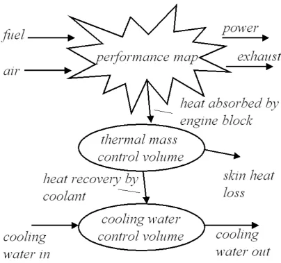
Analysis of performance data from several µ-CHP units coupled with extensive model development and testing work within IEA ECBCS Annex 42 [7, 9] has indicated that the generic form of model shown in Figure 1 is appropriate for the simulation of µ-CHP devices; this was developed using a pragmatic “grey box” modelling approach, where the model structure partially reflects the underlying physical device.

<<figure 1 here>>

The engine unit is represented as a single functional block with a series of inputs and outputs; these are linked by a performance map (a series of parametric equations linking the inputs of the model to the outputs). In addition, the heat output passed to a lumped-capacitance thermal model, featuring two thermal control volumes, which are added to enable the transient thermal performance of the engine unit and coupled heat exchange equipment (engine jacket and exhaust gas heat exchanger) to be adequately modelled. These are:

• the thermal mass control volume that (roughly) represents the aggregated thermal capacitance associated with the engine block and the majority of the heat exchanger shells; and

The need for two control volumes emerged from the analysis of the thermal response of both Stirling and ICE engine units. In both cases the cooling water outlet temperature (this is the coupling point between the device and the rest of an integrated model) exhibited rapid changes to variations in coolant flow rate and temperature and much slower response to changes in engine loading. The two-volume model can adequately represent both of these responses.

2.1 Performance Map

In the performance map, the engine’s steady-state (part load) performance is correlated to the total energy input to the system:

gross e ss

net q

P _, =η ₍₁₎

gross q ss

gen q

q _, =η ₍₂₎

fuel fuel

gross m LHV

q = & ⋅ ₍₃₎

The cogeneration system’s part load electrical and thermal efficiencies, (ηe, ηq [-]), are determined using empirical correlations relating the conversion efficiencies to the flow rate and temperature of cooling water, and the unit’s electrical loading:

) , ,

( _{cw cw net,ss} e = f m& T P

and

) , ,

( _{cw cw net,ss} q = f m& T P

η ₍₅₎

Effectively, this performance map describes the cogeneration system’s steady-state behaviour under a variety of loading conditions.

The full performance map expression for electrical efficiency is as follows:

cw cw ss net cw cw ss net cw cw ss net cw cw ss net cw cw ss net cw cw ss net cw cw ss net cw cw ss net cw cw cw cw cw cw cw cw cw ss net cw ss net cw ss net cw ss net cw ss net cw ss net cw ss net cw ss net cw cw cw cw ss net ss net e T m P a T m P a T m P a T m P a T m P a T m P a T m P a T m P a T m a T m a T m a T m a T P a T P a T P a T P a m P a m P a m P a m P a T a T a m a m a P a P a a & & & & & & & & & & & & & & & & & & , 26 2 , 25 2 , 24 2 , 23 2 2 , 22 2 2 , 21 2 2 , 20 2 2 2 , 19 2 18 2 17 16 2 2 15 2 , 14 2 , 13 , 12 2 2 , 11 2 , 10 2 , 9 , 8 2 2 , 7 6 2 5 4 2 3 , 2 2 , 1 0 + + + + + + + + + + + + + + + + + + + + + + + + + + =

η

Similarly for thermal efficiency:

Where a0–a26 (-) and b0–b26 (-) are empirically-derived coefficients. Many of these coefficients reduce to zero after regression analysis for particular devices, however they have been included for completeness.

Note that the efficiency correlations described by equations 6 and 7 quantify the cogeneration system’s steady-state and part load performance, and do not characterize its dynamic thermal or electrical behaviour.

2.2 Thermal Mass Control Volume

The dynamic thermal behaviour of the a combustion-based cogeneration device is characterized by the thermal mass of its engine block and encapsulated working fluid, internal heat exchange equipment; these are represented using a single, homogeneous thermal mass control volume. The thermal energy stored within this control volume is quantified using an aggregate thermal capacitance, [MC]eng, (J/K) and an equivalent average engine temperature Teng (oC).

The energy balance of the thermal mass control volume shown in figure 1 is:

loss skin HX ss gen eng

eng q q q

dt dT

MC] = _, − − ₋

[ (8)

2.2.1 Cooling water control volume

The energy balance of the cooling water control volume shown in figure 1 is:

(

)

cw p o

cw

cw mc T T q

dt T

MC , = _, − _, +

] [ ]

[ & (9)

• the thermal mass of the engine and other heat transfer components , which store some of the recoverable heat produced within the engine, and

• the effects of internal controllers regulating phenomena such as of exhaust-gas recirculation and the operation of an external heater in Stirling engines.

The heat transfer between the engine and the cooling water control volume is quantified using an overall heat-transfer coefficient:

(

)

HX

HX UA T T

q = − _{, (10)}

It is assumed that the heat lost from the engine is proportional to the temperature difference between the engine and the surroundings. Thus:

(

)

loss loss

skin UA T T

q ₋ = − (11)

where UAloss (W/K) is the effective thermal conductance between the engine control volume and the surroundings.

Using Equations 10 and 11, the engine and cooling water control volume energy balance equations (Equations 8 and 9) can be rewritten:

(

)

(

)

eng

eng UA T T UA T T q

dt dT

MC] _{, ,}

[ = − + − +

(12)

(

)

(

)

cw p o

cw

cw mc T T UA T T

dt T

MC] , [ ] _{, , ,}

3 MODEL CALIBRATION

Calibration of the parameters for this model is a two stage process. The first stage is to produce the performance maps that characterise the performance at different operational states: different loading levels (where appropriate), cooling water flow rates and temperatures. The main function of the performance map is to predict the heat transferred to the cooling system of the unit; it is also used to predict the unit’s fuel consumption.

3.1 Dynamic Calibration

The second stage of the calibration process was to tune the characteristics (MCeng, MCcw, UAHX and UAloss) of the dynamic thermal model using data from dynamic tests on the µ-CHP unit; these tests could cover periods when the unit is in start-up or shut down mode and/or when the thermal or electrical load on the unit is changed.

The necessary performance maps (equations 6 and 7) were developed by regression

analysis using data from laboratory tests in which the µ-CHP unit was tested at

various load levels and cooling water flow rates.

Calibration of the dynamic elements of the model (control volumes) required an iterative parameter identification procedure using the GenOpt optimization utility (Wetter [10]); this is designed to determine the parameter set providing the minimum value of a specified cost function; in this case this is the average error between the measured cooling water outlet temperature and the value predicted by the model:

∑

=

=

=

N i

i i e N E

1

1 (25)

3.2 Stirling Engine Calibration and Validation

Calibration of the Stirling Engine was undertaken by Ferguson [9] using the two-stage process described with data collected by Entchev et al. [11], who installed a small, Stirling CHP unit an experimental test house at the Canadian Centre for Housing Technology (CCHT), and measured its performance when subjected to simulated thermal loads. This data set was split into two: one set was used for calibration and

the other for verification of the model’s predictions. The Stirling µ-CHP unit used in

this study exhibited relatively low electrical efficiency (8-9% LHV), and a high heat-to-power ratio (9:1). The unit had a 750We electrical output and was capable of producing around 7 kW of heat. The device was regulated using an on-off controller and exhibited nearly constant fuel flow and electrical output when operating.

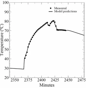
Figure 2 plots the Stirling µ-CHP model’s predictions against experimental data for a two-hour test period. In this test, the unit was started from cold and the coolant flow rate perturbed. The test was replicated with the model and the results indicate that it can adequately represent the dynamic performance of the unit.

<<figure 2 here>>

3.3 ICE Calibration

A similar process was undertaken to calibrate the model to steady-state and dynamic performance data from a Senertec ICE unit. This unit has different characteristics to the Stirling Engine in that it has a peak electrical power output of 5 kW and a thermal output of 14.5 kW. The predictions of the calibrated model in comparison to experimental tests (in which the unit is switched on and off and the coolant flow rate is varied) are shown in figure 3. Again, this shows that the calibrated generic model gives a good prediction of the dynamic thermal performance of this µ-CHP device.

4 CASE STUDY

Using the building simulation tool equipped with the µ-CHP device model the energy

and environmental performance (e.g. CO2 emissions and fuel consumption) of a Stirling engine-based domestic heating system was determined when integrated into a detached dwelling. Further, as befits the detailed nature of the model developed, more fine-grained performance data was also examined: on/off cycling, transient thermal performance, the impact of balance of plant and the temporal characteristics of

electrical output. Using this information, the potential for the µ-CHP to actively

participate with the local electrical network in areas such as voltage control was assessed.

4.1 Integrated Model

Building Fabric

The ESP-r building model was developed from various analyses of the UK housing stock [12,13,14] and comprises a representation of the building geometry coupled with explicit representations of the different constructions, occupancy characteristics, temporal hot water draws along with space and water heating control requirements. The total floor area of the dwelling is 136 m2.

the model when they were used. These two levels of insulation bracket the range of

dwelling fabric types within which a µ-CHP unit could be expected to operate.

Occupancy

The dwelling model was populated by a four-person family. Corresponding detailed daily heat gain profiles (covering weekdays and weekends) for people and equipment based on continuous occupancy and intermittent occupancy were developed based on the work of Jardine [15].

Heating System

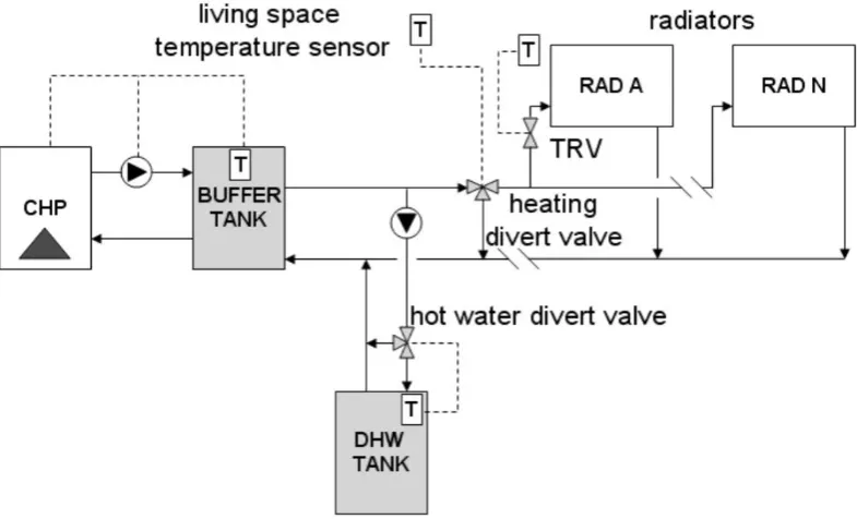
The detailed model of the heating system, which was integrated with the building

model is shown in figure 4. The µ-CHP unit was coupled to the rest of the heating system via a 200l buffer tank featuring an internal heat exchanger: this fed both the

radiators and the domestic hot water tank and buffers the µ-CHP unit from the

instantaneous space heat and hot water demands, reducing the need for on/off cycling. The core of the system and the buffer tank capacity is typical of that seen in

demonstration installations for µ-CHP, e.g. Entchev et al. [11].

<<figure 4 here>>

4.2 Simulations

Four variants of the dwelling model were developed featuring different combinations of fabric insulation and occupancy. For each, two simulations were run representing a typical heating season week in winter and the transition seasons (spring/autumn). These used a London data set (the reference UK dynamic climate for building simulations). Each simulation was conducted using a 5-minute time step, enabling the dynamics associated with the thermal inertia of components and the operation of the various controllers in the dwelling’s heating system to be captured.

The simulations run are labelled as follows:

• transition #11 – transition week, poorly insulated, continuous occupancy;

• winter #11– winter week, poorly

insulated, continuous occupancy;

• transition #12 – transition week, poorly insulated, intermittent occupancy;

• winter #12 – winter week, poorly insulated, intermittent occupancy;

• transition #21 – transition week, well insulated, continuous occupancy;

• winter #21– winter week, well

insulated, continuous occupancy;

• transition #22 – transition week, well insulated, intermittent occupancy;

4.3 Results

Figure 5 gives a sample of some of the large quantity of detailed, dynamic performance information available from the building simulations. It shows the water temperature in the buffer tank, the associated µ-CHP electrical power output and the temperature in the living room of the dwelling over the course of a simulated week. For this paper, systems-level summary performance metrics have been extracted from the detailed simulation data. This is presented in tables 2-6. These tables summarise the overall energy performance of the µ-CHP system and characterise some of the temporal characteristics relevant to its mechanical performance and availability to provide services to the local electrical network.

<<figure 5 here>>

4.4 Discussion of Results

Energy and Environmental Performance

The impact of adequately insulating the building reduced the space heating requirements by up to 60% and also had a significant impact on the effectiveness of

the Stirling µ-CHP system. In all of the simulations the basic device efficiency was

extremely good, ranging from 88% up to 95%. The higher device efficiencies occurred during the winter week, and corresponded to the heaviest heat loading. Unit efficiencies fell in the transition week and also as the insulation level of the dwelling increased; this was due to greater unit cycling frequencies and a reduction in the time in which the unit was producing power.

the buffer tank, hot water tank and piping. The effect was even more pronounced for the well-insulated dwelling, with system efficiencies ranging from 18 to 40% lower than the device efficiency. The poorest performance occurred during the transition week, when the useful heat load was reduced in comparison to the parasitic losses: in this situation more heat was lost from the tanks and piping than was usefully delivered to the space. In winter this effect was less pronounced as the space heating demands were higher.

It is interesting to note that the high µ-CHP device and system efficiencies occurred in

the ‘winter #11’ and ‘winter #12’ simulations for the poorly insulated dwelling. However, closer inspection of the simulation results indicated that the heating system supply and hot water tank temperatures were often lower than the required system set point temperatures and so the system heat losses were lower than would otherwise be the case. Hence, although the derived efficiency was high, the system failed to deliver enough heat to provide thermal comfort in the dwelling at certain times. The same problem occurred (though to a lesser extent) in the transition #12 simulation.

Temporal Characteristics

The mode of operation, the season and insulation levels had a significant impact on

cycling frequency would be beneficial to the longevity of the µ-CHP device and

would reduce maintenance.

When heavily loaded, the unit tended to operate for long periods on full power in an attempt to maintain the buffer tank temperature within the operating range of 65-75oC. However, with a lighter heat load the buffer tank reached its operating conditions more quickly and then the µ-CHP unit cycled to stay within the

temperature range. The number of cycles was similar for each transition period simulation (transition #11 and #21). However, the average unit on time was reduced from an average of 296 minutes to 157 minutes with better dwelling insulation levels.

The number of operational cycles and their length directly affected the amount of

power produced by the µ-CHP unit. As the heat demand fell so did the potential for electricity cogeneration, for example during the winter week the electrical output of the Stirling unit was 118 kWh however this dropped to 57 kWh for the better-insulated case.

When the heating system was operated intermittently in winter to complement an intermittent occupancy, the number of cycles did not vary between simulations. The constrained unit operation time resulted in the unit being on when the control regime allowed as between the intermittent firing, the buffer tank temperature fell below the minimum set point temperature of 65oC due to parasitic heat losses. Hence, in the next operational period the unit needed to fire continuously to bring the tank temperature back into the operating range.

dwelling reduced this to 25% of the time, with a corresponding reduction in electrical production from 48kWh to 31kWh. The difference was far less pronounced for the winter simulation. Operational times only fell from 40% to 38%. This was symptomatic of the intermittent control rather than a true reflection of the effect of insulating the dwelling. As was mentioned previously, for the poorly insulated,

intermittent winter case (winter #12), the µ-CHP system struggled to achieve the

operating temperature range in the buffer tank, so the actual operating time would have been significantly longer than the 40% observed if the device had not been constrained by the control settings.

Availability for Participation in HDPS Control

The ability to externally control a µ-CHP device to meet some network need could be

an important element in the safe and reliable operation of an HDPS. However the ability of the device to respond to such a need is heavily constrained by the thermal demands of its client building. The data from the simulation results was analysed to

give an indication of likely ability of the µ-CHP to respond to an external network

control signal. For the non-modulating device modelled, three responses to external requests for control were possible:

1. If the buffer tank temperature was below its upper limit of 75oC and the device is off then the it could be switched on to provide power to the network (i.e. to counteract a drop in the network voltage) until the upper temperature limit of the buffer tank was reached – positive participation.

3. Finally if the device was on with a buffer tank temperature of below 65oC or off with a buffer tank temperature of above 75oC then the unit was unavailable for use in network control as the dwelling’s thermal needs had priority - unavailable.

Note that in cases 1 and 2 the thermal loads in the dwelling would continue to be served by the buffer tank and were be unaffected by the external control of the unit.

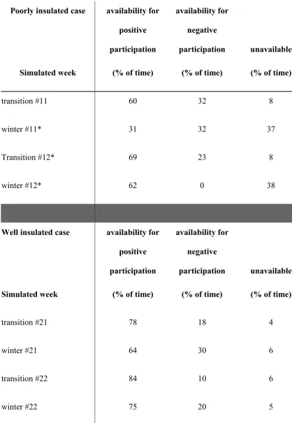
Table 6 shows the resulting µ-CHP device availabilities from each simulation - typically above 90%. However, in cases where the device struggled to meet the heat load (the poorly insulated dwelling in winter) availability reduced to around 60% as the device would often was on with a buffer tank temperature of below 65oC. The participatory mode was influenced by the level of insulation: in the well insulated ‘Passivehaus’ dwelling availability for negative participation (i.e. switching off) was markedly less than for the poorly insulated dwelling (figure 7) due to the smaller dwelling heat load and reduced run time for the unit. Conversely, scope for positive HDPS participatory (switching on from standby) control was increased.

Determining the Duration of Participation

An analysis of the buffer tank thermal characteristics from the simulations indicated that its typical cool down time from 75oC to 65oC was around 800 minutes. The heating time between the same temperature bands was approximately 200 minutes. Using this information it was possible to derive the approximate time for positive or

negative participation of the µ-CHP device for any point in time during a simulation.

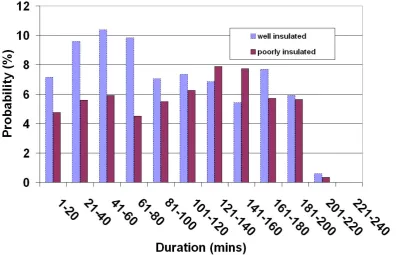
ranged from 1 to 200+ minutes. However, increasing the insulation levels significantly increased the probability of participation times lasting less than 100 minutes.

<<figure 6 here >>

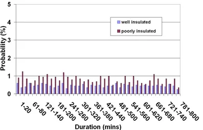
Figure 7 shows the corresponding probabilities for negative participation for different participation duration times, which ranged from 1 to 800+ minutes. These were significantly lower over the spectrum of duration times than was the case for positive participation. Increasing insulation levels reduced these probabilities further.

<<figure 7 here>>

5 CONCLUSIONS

This paper has described the development and testing of a generic µ-CHP device

model for use in integrated simulations of domestic energy systems. The model uses a modified performance-map to enable the calculation of the part load performance. This is combined with a dynamic thermal model comprising two lumped thermal masses enabling the device model to adequately capture the dynamic variations of the cooling water temperature: the critical thermal coupling variable between the device, heating system and client building. The model has been calibrated to represent both

Stirling and internal combustion engine-based µ-CHP devices.

The performance of the micro-CHP system deteriorated when dwelling insulation levels were improved. However, reduced heat demands led to an overall reduction in carbon emissions. Better dwelling insulation also reduced the electrical power produced by the unit and therefore the potential to displace grid electricity or export power to the grid.

When considering the potential for provision of network services from the micro-CHP device it was found that the device was generally available around 90% of the time to respond to a request from the network service in cases where the device struggled to meet the thermal load of the dwelling. In these cases availability was significantly lower.

The device could switch off in response to an external control signal for between 1 to 800+ minutes and switch on for between 1 to 200+ minutes. In both cases the maximum response time depended upon the tank temperature and prevailing heat loads. Improving the insulation level of the dwelling significantly increased the availability of the device to switch on and provide power to the network (i.e. to raise voltage levels). The availability of the device to a switch off signal from the network remained low for both the well insulated and poorly insulated cases.

Finally, the results from the simulations demonstrated the strong couplings between the µ-CHP system, the balance of plant and the load thus emphasising the value of

fully integrated modelling as described in this paper.

5.1 Further Work

This paper here has dealt mainly with the development of a generic µ-CHP device

context. The device model and building simulation will be applied to a much broader range of devices, dwellings, climates and operational scenarios to produce a more comprehensive picture of performance in the UK housing stock as a whole.

6 ACKNOWLEDGEMENTS

The model development and calibration described in this paper was undertaken as part of the International Energy Agency’s Energy Conservation in Building and Community Systems research Annex 42: The Simulation of Building- Integrated Fuel Cell and Other Cogeneration Systems (www.cogen-sim.net). The Annex is an international collaborative research effort and the authors gratefully acknowledge the indirect or direct contributions of the other Annex participants.

The simulation work described in this paper was undertaken within the SuperGen Highly Distributed Power Systems consortium. The authors gratefully acknowledge the funding and support of the UK Engineering and Physical Sciences Research Council and the indirect or direct contributions of the other consortium members.

7 NOMENCLATURE

e

η

q

η the steady-state part load, thermal efficiency of the engine (-)

fuel

LHV the lower heating value of the fuel used by the system (J/kg or J/kmol)

fuel

m& the fuel flow rate (kg/s or kmol/s),

cw

cw

T the temperature of the cooling water at the inlet of the cooling water control volume (oC).

kf an empirical coefficient (-)

up warm fuel

m& _{, −} the rate of fuel flow during warm-up (kg/s)

max ss fuel m& _{, −}

(kg/s)

the maximum rate of fuel flow to the device under steady-state conditions (kg/s)

cw p

c

m& the thermal capacity flow rate associated with the cooling water (W/K)

eng

MC the thermal capacitance of the control volume (W/K)

cw

MC the thermal capacitance of the encapsulated cooling water and heat exchanger shell in immediate thermal contact (J/K)

ss net

P _, is the rate of steady-state electricity production (W)

ss gen

q _, the steady-state rate of heat generation within the engine (W)

gross

q is the gross heat input into the system (W)

HX

q the rate of heat transfer to the cooling water (W)

loss skin

q ₋ the rate of heat loss from the unit (W)

o cw

i cw

T _, the temperature of the cooling water entering the unit (oC)

eng

T the bulk temperature of the thermal mass control volume (oC)

t time (s)

Teng the average temperature of the engine control volume. (oC)

Teng,nom the nominal engine temperature (oC)

UAHX the overall thermal conductance between the engine cooling water control volumes (W/K)

8 REFERENCES

1 Burt G, 2008. An Overview ofThe Highly Distributed Power System Concept, Proc Microgen 2008, The First International Conference and Workshop on Micro-cogeneration and Applications, National Arts Centre, Ottawa, Canada, Apr 29-May 1

2 Dentice d'Accadia M, Sasso M, Sibilio S, Vanoli L, 2003. Micro-combined heat and power in residential and light commercial applications, Applied Thermal Engineering, 23 (10) 1247-1259

3 Slowe J, 2008.International Micro-CHP Review and Outlook, Proc. Microgen2008, The First International Conference and Workshop on Micro-cogeneration and Applications, National Arts Centre, Ottawa, Canada, Apr 29-May 1

5 Peacock A, Newborough M, 2005. Impact of micro-CHP systems on domestic sector CO2 emissions. Applied Thermal Engineering, Volume 25, Issue 17-18, pp 2653-2676.

6 Cockroft J, Kelly N J, 2006. A Comparative Assessment of Future Heat and Power Sources for the UK Domestic Sector, Energy Conversion and Management 47, pp 2349-2360.

7 Beausoleil-Morrison I, Kelly N J, eds., 2007. Specifications for Modelling Fuel Cell and Combustion-Based Residential Cogeneration Device within Whole-Building

Simulation Programs, IEA/ECBCS Annex 42. Available at www.cogen-sim.net.

8 Clarke J A 2001. Energy Simulation in Building Design, 2nd Ed, Butterworth-Heineman, London.

9 Beausoleil-Morrison I. and Ferguson A., eds., 2007. Inter-model Comparative Testing and Empirical Validation of Annex 42 Models for Residential

Cogeneration Devices, IEA/ECBCS Annex 42. Available at www.cogen-sim.net.

10 Wetter M, 2004. GenOpt(R) Generic Optimization Program, Lawerence Berkeley National Laboratory, US Deparment of Energy.

11 Entchev E, Gusdorf J, Swinton M, Bell M, Szadkowski F, Kalbfleisch W and Marchand R 2004. Micro-generation technology assessment for housing technology, Energy and Buildings, 36(9), September, pp925-931.

12 Department for Communities and Local Government, English House Condition Survey 2004 (http://communities.gov.uk/ehcs )

14 Utley J I, Shorrock L, Brown J H F, 2001. Domestic Energy Fact File: England, Scotland, Wales and Northern Ireland, BRE Report Available at www.bre.co.uk

15 Jardine C, Synthesis of High Resolution Domestic Electricity Load Profiles, 2008. Proc Microgen2008, The First International Conference and Workshop on Micro-cogeneration and Applications, National Arts Centre, Ottawa, Canada, Apr 29-May 1

16 Jordan U and Vajen K 2000. Influence of the DHW Load Profile on the Fractional Energy Savings: A Case Study of a Solar-combi System with TRNSYS

Simulations, Solar Energy (69), pp 197-208.

9 TABLES

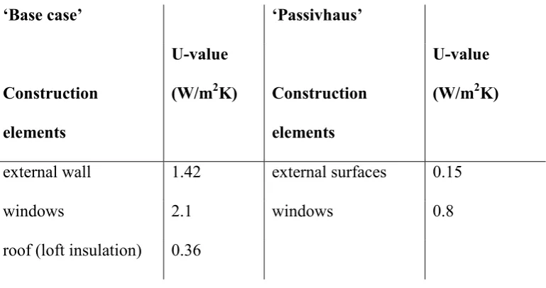
Table 1: U-values used in building models.

‘Base case’ ‘Passivhaus’

Construction elements

U-value

(W/m2K) Construction elements

U-value (W/m2K)

external wall 1.42 external surfaces 0.15

windows 2.1 windows 0.8

roof (loft insulation) 0.36

Table 2: energy and environmental metrics for µ-CHP from simulations, poorly-insulated dwelling.

Poorly insulated

Unit eff.

Net Power

Heat

out Losses CO2

Space heat

Water

heat Sys eff.

Simulated

week (%) KWh kWh KWh kg kWh kWh (%)

transition #11 92 73 690 150 186 445 95 74

winter #11 95 118 1025 165 269 768 93 82

transition #12 92 48 466 49 126 357 59 83

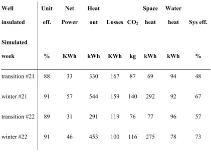
Table 3: energy and environmental metrics for µ-CHP from simulations, well-insulated dwelling over a simulated week.

Well insulated

Unit eff.

Net Power

Heat

out Losses CO2

Space heat

Water

heat Sys eff.

Simulated

week % KWh kWh KWh kg kWh kWh %

transition #21 88 33 330 167 87 69 94 48

winter #21 91 57 544 159 140 292 92 67

transition #22 89 31 291 119 76 77 96 57

winter #22 91 46 453 100 116 275 78 73

Table 4 temporal metrics for µ-CHP from simulations with poorly-insulated dwelling over a simulated week.

Poorly insulated % of time % of time ave time ave time cycles

Simulated week

on/

warmup

standby/

cool down

on

mins

Standby

Mins #

transition #11 59 41 296 199 20

transition #12 40 60 266 407 15

winter #12 40 60 266 407 15

Table 5: temporal metrics for µ-CHP from simulations with well-insulated dwelling over a simulated week.

Well insulated % of time % of time ave time ave time cycles

Simulated week

on/ warmup

standby/ cooldown

on mins

Standby

mins #

transition #21 28 72 157 403 18

winter #21 46 54 222 247 21

transition #22 25 75 166 506 15

Table 6: Availability of the µ-CHP to participate in HDPS control.

Poorly insulated case availability for positive participation

(% of time)

availability for negative participation

(% of time)

unavailable

(% of time) Simulated week

transition #11 60 32 8

winter #11* 31 32 37

Transition #12* 69 23 8

winter #12* 62 0 38

Well insulated case availability for positive participation

(% of time)

availability for negative participation

(% of time)

unavailable (% of time) Simulated week

transition #21 78 18 4

winter #21 64 30 6

transition #22 84 10 6

winter #22 75 20 5

CAPTIONS FOR FIGURES

Figure 3: ICE model predictions of cooling water temperature vs. experimental results

Figure 5: Sample of results available from the simulations.