Integrating cluster formation and cluster evaluation in interactive visual analysis

City, University of London Institutional Repository

Citation

:

Turkay, C., Parulek, J., Reuter, N. and Hauser, H. (2011). Integrating cluster

formation and cluster evaluation in interactive visual analysis. Paper presented at the 27th

Spring Conference on Computer Graphics, 28 Apr - 30 Apr 2011, Vinicne, Slovakia.

This is the accepted version of the paper.

This version of the publication may differ from the final published

version.

Permanent repository link:

http://openaccess.city.ac.uk/3618/

Link to published version

:

Copyright and reuse:

City Research Online aims to make research

outputs of City, University of London available to a wider audience.

Copyright and Moral Rights remain with the author(s) and/or copyright

holders. URLs from City Research Online may be freely distributed and

linked to.

City Research Online:

http://openaccess.city.ac.uk/

[email protected]

Integrating Cluster Formation and Cluster Evaluation

in Interactive Visual Analysis

Cagatay Turkay∗ Department of Informatics

University of Bergen

Julius Parulek†

Department of Informatics University of Bergen

Nathalie Reuter‡

BCCS University of Bergen

Helwig Hauser§

Department of Informatics University of Bergen

Abstract

Cluster analysis is a popular method for data investigation where data items are structured into groups called clusters. This analysis involves two sequential steps, namely cluster formation and cluster evaluation. In this paper, we propose the tight integration of cluster formation and cluster evaluation in interactive visual analysis in or-der to overcome the challenges that relate to the black-box nature of clustering algorithms. We present our conceptual framework in the form of an interactive visual environment. In this realization of our framework, we build upon general concepts such as cluster com-parison, clustering tendency, cluster stability and cluster coherence. Additionally, we showcase our framework on the cluster analysis of mixed lipid bilayers.

CR Categories: I.3.m [Computing Methodologies]: Computer Graphics—Miscellaneous; H.3.3 [Information Storage and Re-trieval]: Information Search and Retrieval—Clustering

Keywords: Visual Analysis Models, Visual Knowledge Discov-ery, Data Clustering, Bioinformatics Visualization.

1

Introduction

Cluster analysis divides data into groups (clusters) where data items within a group are similar with respect to certain criteria. Usu-ally, data items are clustered using solely the information which is available in the data which represents the items and their relations. Clusters provide the analyst with a grouping structure without pro-viding any information on why they exist and which properties they have (e.g., whether the clustering is stable) [Tan et al. 2006]. Con-ventionally, cluster analysis involves two consecutive steps;cluster formationandcluster evaluation. Cluster formation is a black-box operation where the user specifies a clustering algorithm together with a set of parameters and gets an according clustering. Here, we refer to clustering as the entire set of clusters. Usually, the forma-tion step is followed by an evaluaforma-tion phase where the user decides whether she is satisfied with the clustering, or not. If the results are implausible, the process is carried out again with a different param-eter set and/or algorithm.

∗_{e-mail: [email protected]}

†_{e-mail:[email protected]}

‡_{e-mail:[email protected]}

§_{e-mail:[email protected]}

Assessing a clustering’s quality and fine tuning the clustering algo-rithms are complex tasks due to the following facts [Tan et al. 2006]. Firstly, the relations in the data that eventually lead to a cluster-ing vary from domain to domain. This makes it hard to generalize and formalize the definition of what a valid cluster is. Secondly, clusters do not usually reveal any implicit information on data rela-tions, making them harder to be interpreted. Thirdly, clustering al-gorithms are highly dependent on their parameters and often these parameter sets do not offer a good basis for the analyst to steer the analysis using her domain knowledge. There is a certain need for mechanisms to enhance cluster analysis. These mechanisms should include a stronger utilization of the analyst’s domain knowledge in cluster analysis together with methods for the interactive analysis of raw data (together with the clusters). Such mechanisms would not only lead to more satisfactory clusterings but also provide more insight into the underlying relations in data. This insight eventually increases the confidence of the expert on cluster analysis results.

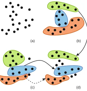
As an illustration of a situation where integration of the expert in cluster analysis is required, let us assume a demonstrational case (Fig. 1), where points are scattered on a 2D plane without any structurally apparent clustering. With a slight change in input

pa-(a) (b)

(c) (d)

Figure 1: Ambiguity in the cluster analysis of a set of 2D points a) Initial set of points; b),c) Two possible clustering results; d) The re-sulting clusters obtained by a combination of the original two clus-terings, where regarding one cluster there is a need to change the cluster by removing some points (dashed arrow).

rameters, two runs of a clustering algorithm can result in different clusterings (Fig. 1b,c). After the evaluation phase, the analyst can reckon that both clusterings are unsatisfactory. However a combi-nation of both results, which is not necessarily the outcome of any clustering algorithm, could be a satisfactory clustering (Fig. 1d). In order to resolve this ambiguity, the analyst needs to steer the cluster formation process by using a combination of her domain knowledge and the insight gained throughout the analysis.

fun-damental subset of these techniques relate toclustering tendency,

cluster comparison, cluster stabilityand cluster cohesion. Clus-tering tendency reveals if there is a non-random structure in the selected data sample [Smith and Jain 1984]. An apparently struc-tured sample would lead to a successful clustering much more than a sample with almost a random structure. Ideally, cluster analysis begins with the evaluation of the clustering tendency of the inves-tigated data. Cluster comparison is a clear requirement of cluster analysis owing to the fact that clustering algorithms are often quite stochastic and parameter dependent [Jain 2010]. Cluster analysis does not usually rely on a single result of a particular algorithm. Analysts make a number of different clusterings with different pa-rameters (and algorithms). Intuitive and interactive mechanisms to compare clusters need to be a part of any cluster analysis process. Cluster stability and cluster cohesion are important criteria to eval-uate the validity of a cluster. A cluster can be considered stable when its members are generally clustered together in different clus-terings [Lange et al. 2004]. Cluster cohesion, on the other hand, depicts how tight the items are in a single cluster [Tan et al. 2006]. It is possible to observe additional structures in a cluster with low cohesion. Analysts can reckon that an unstable and/or an incoherent cluster is not valid and that it requires a refinement. Conventional cluster analysis employs these techniques separately in the steps of cluster formation and cluster evaluation in order to achieve high quality clusterings [Tan et al. 2006]. However, we are not aware of any solution which integrates these techniques in an interactive and iterative analysis procedure.

To achieve this, we describe a framework that tightly integrates cluster formation and cluster evaluation in interactive visual anal-ysis (IVA). In cluster formation we employ the explorative power of the human perception to discover subsets of the data with higher clusteringtendency. In cluster evaluation, we utilize the expert’s domain knowledge tocompare and evaluate clusters in terms of theirstabilityandcohesion.

In this paper, we also realize and present the proposed framework in the form of an interactive visual environment. In this environment, we incorporate conventional views as well as two specific views for the two aforementioned purposes. The conventional views are scatter plots, histograms and function graphs which are used in link-ing&brushing operations. The two more special views are acluster tendency viewto evaluate the suitability of data subsets for cluster-ing and aparallel cluster viewto interact with a number of different clusterings and to compare them. Importantly, in all the stages of the analysis, clusters are treated as an additional dimension of the actual dataset. This approach enables us to tightly integrate clusters in the IVA cycle.

Keim et al. [Keim et al. 2008] stated that an important task of visual analytics is to integrate the knowledge, explorative power and cre-ativity of the human with the computational power of algorithms. We follow this research goal with the visual exploration and anal-ysis of clusterings which not only enable experts to discover more reliable groupings in data but also provide information on why these groupings exist at all.

2

Related Work

Interactive techniques have proven to help analysts to manually refine and build clustering results. A hierarchical clustering and visualization algorithm, H-BLOB, is introduced by Sprenger et al. [Sprenger et al. 2000]. The authors propose a visual clustering approach which involves a two-stage procedure, where a hierarchi-cal clustering is followed by a visualization, using blob objects, to

reveal cluster shapes. Rinzivillo et al. use a visually driven tech-nique called progressive clustering [Rinzivillo et al. 2008] where the clustering is done in successive steps using different distance functions. The authors show that the progressive clustering tech-nique provides a convenient mechanism, where a user can selec-tively direct the algorithms to potentially interesting portions of data. Schreck et al. [Schreck et al. 2008] propose a framework to interactively monitor and control Kohonen maps to cluster trajec-tory data. In their paper, they state the importance of integrating the expert in clustering process to achieve suitable results.

Visualization has generally served as the final step of cluster anal-ysis where it plays a critical role in enhancing the interpretation of clusters by enabling comparison and evaluation. Grottel et al. [Grottel et al. 2007] use interactive visual tools to analyze clus-ters in molecular dynamics. The authors introduce the concept of flow groups, which display cluster evolution over time, to val-idate the quality of clustering results. In a recent study, Rubel et al. [Rubel et al. 2010] introduce a framework that integrates clus-tering and visualization for the analysis of 3D gene expression data. Authors integrated the data clustering for 3D gene expression anal-ysis into their PointCloudXplore visualization tool. The approach in this study is application oriented, therefore enables only a lim-ited utilization. On the contrary, our framework can be applied to arbitrary multivariate and/or time varying datasets.

InHierarchical Clustering Explorer[Seo and Shneiderman 2002], Seo and Shneiderman use an interactive dendogram coupled with a color mosaic to represent clustering information together with conventional visualizations. They also include a cluster compari-son view where the user can compare two clustering results. In a recent study, Lex et al. introduce MatchMaker [Lex et al. 2010], where they visualize and compare multiple groups of dimensions. In their work, they provide a use-case where they use their methods to compare clusters. We enrich this cluster comparison capability by mechanisms to compare clusters not only on member items but also on quality. Vectorized radial visualizations are used in explor-ing different clusterexplor-ing results by projectexplor-ing data records on a vec-torized cluster space [Sharko et al. 2008]. This approach proves to be useful in validating the clusters when many different clusterings for the same dataset exist. An interactive dissimilarity matrix, pre-sented by Bezdek and Hathaway [Bezdek and Hathaway 2002], was extended to analyze clustering results at different similarity level by Siirtola [Siirtola 2004]. Sharko et al. [Sharko et al. 2007] use heat maps called cluster stability matrices to visually analyze and re-veal most ’stable’ clusters in clustering results. In our approach, we enhance the cluster comparison capability in the above stud-ies [Seo and Shneiderman 2002] [Sharko et al. 2008] by using IVA operations in the parallel cluster view. Moreover, we enhance and integrate the dissimilarity matrix [Bezdek and Hathaway 2002] vi-sualizations with cluster comparison plot in an interactive visual analysis cycle to fill the gap between cluster evaluation and cluster formation in cluster analysis.

3

Integrating Cluster Formation and

Clus-ter Evaluation

Clustering Tendency Domain

Selection

Integrated Clustering

Cluster Formation

Cluster Stability

Clustering Comparison

Cluster Coherence

+ Cluster Evaluation

(1)

(4)

(3) (2)

(5)

C0 C1

...

...

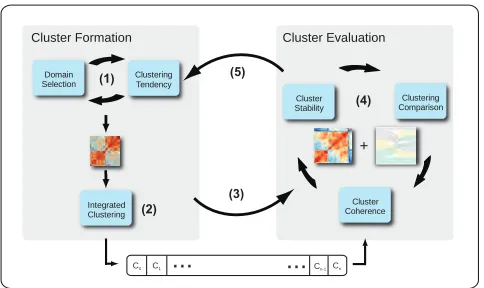
Figure 2: An illustration of our framework. Iterative exploration is performed to find suitable data subsets for clustering (1). Suitable selections are clustered and stored (2). Analysis continues with the evaluation phase (3). Evaluation is carried out in an IVA cycle by comparing clusters with respect to their stability and coherence (4). Analysis continues by incorporating the insight from the evaluation phase (5).

for a clustering (Fig. 2-1). Here, the domain refers to brushed items and a set of dimensions to use in clustering. The selected domains are evaluated with respect to their tendency for clustering by using the cluster tendency view. The selected domain is then clustered using one of the clustering methods and the resulting clusterings are stored (Fig. 2-2). Cluster analysis continues with the evaluation phase (Fig. 2-3). This phase is performed using the cluster tendency view and the parallel cluster view together with conventional visu-alization support (Fig. 2-4). In this phase, the parallel cluster view is used to assess cluster stability and to compare clusters. Addition-ally, when used in conjunction with the cluster tendency view, it provides a mechanism to discover cluster coherence. Cluster analy-sis is iteratively continued using the insight gained in the evaluation phase (Fig. 2-5).

In the realization of our conceptual framework we follow the data model presented by Konyha et al. [Konyha et al. 2006], which pro-vides a suitable and flexible language for the analysis of arbitrary data types. We define the data set of independent variables (items)

asO={o1, . . . ,on}, where each item has a set ofm=p+q

depen-dent valuesF(oi) = [f1(oi), . . . ,fp(oi),gp+1(oi,t), . . . ,gp+q(oi,t)],

wherefrepresents regular andgrepresents temporal variables. The regular variables have a singular value for each oi and temporal

variables change their values over a time interval. We define the clustercasc⊆Oand the clusteringCas a set of clustersC⊆2O, where the following clustering criteria hold:

[

c∈C

⊆Oand∀ca,cb∈C:ca6=cb⇒ca∩cb=/0. (1)

Note that in (1) we do not expect clusteringCto include all the items inO. This is firstly due to the fact that clusterings can be performed on non-overlapping subsets of the data and secondly that data can contain outlier items which are not possible to include in a cluster.

Our conceptual framework is realized in the visual environment named CIVA (Interactive Visual Cluster Analysis). CIVA incor-porates different types of conventional visual analysis views: his-tograms, scatter plots, parallel coordinates, etc. for regular ables; functions graphs and animated scatter plots for temporal vari-ables. Function graph displays allg(o,t), withx-axis as time and

y-axis as the function values. For a better overview of temporal

variables, we implement an animated scatter plot where displayed points move while an internal time variable changes. All of these views are linked through a brushing mechanism, except the ani-mated point graph. This brushing mechanism is similar to compos-ite brushingproposed by Allen and Ward [Martin and Ward 1995]. The result of brushing applied on a view isb⊆O, which is then combined with existing brushes by the boolean operatorSbeing

S∈ {∪,∩,¬}, where∪represents union,∩represents intersection

and¬represents not operator. Every brushbis combined with the previousbiby applying theSoperator:bi+1=S(bi,b). In addition

to the existing brushing scheme, we append a brushing operator on cluster level represented asb=c∈C. For simplicity, in the follow-ing we will denote the final set of brushed items asbL. Moreover,

brushes on temporal variables select a time interval in addition to a list of items. This enables the analyst to concentrate on different time intervals while doing the analysis.

To demonstrate our framework in the following sections, we em-ploy the Iris dataset [Fisher 1936], which is extensively used in data mining literature. The dataset consists of 150 samples from the three species of Iris flowers (Iris Setosa, Iris Versicolour, and Iris Virginica), where four features were measured from each sam-ple, here being our regular variables. The measured features are the sepal length (f1), the sepal width (f2), the petal length (f3) and the

petal width (f4). All the figures up-to Section 5 are visualizations

of this dataset.

3.1 Cluster tendency view

An inherent problem in cluster formation is an assessment of cluster tendencies. Transforming to our IVA viewpoint, the question would be whether the current selectionbLcontains any cluster tendencies.

One of the cluster tendency evaluations is based on visualizing the similarities between items.

To visualize cluster tendencies, we proposeCluster Tendency View

(tendency view), which is based on the dissimilarity matrix visual-ization approach presented by Bezdek and Hathaway [Bezdek and Hathaway 2002]. In the dissimilarity matrix,M, every elementmi,j

represents dissimilarity measure between the itemsoiandoj, which

is smaller for more similar items. Here, for every matrix element, we compute the sum of mutual distances between each pair of vari-ables. Importantly, the matrix is computed not for every item, but only forbL, for which we define dissimilarity matrixMas follows:

mi,j= p

∑

wk∗d fk(oi),fk(oj)

+

q+p

∑

wk∗ "

∑t1

t=t0d gk(oi,t),gk(oj,t)

t1−t0

#

, (2)

whered(·,·)is a distance function,wkare weights that are

spec-ified by the user which can emphasize or suppress (zero) certain variables. Distance functions are essential elements of cluster anal-ysis and there is a large number of distance functions proposed in the literature [Shi et al. 2009]. Especially with time dependent vari-ables, distance function definition should consider domain specific criteria. In this paper, Euclidean distance is preferred ford(·,·).

However, our methods are not bound to a specific distance function andd(·,·)should be chosen to fulfill domain specific constraints

prior to analysis. Time dependent variablesgare computed within the given time interval[t0,t1]. This time interval is interactively

determined by the logical combination of temporal brushes.

Importantly, on every change of the selectionbLor a weight wi,

visual-ized in tendency view. This mechanism enables the tight integra-tion of tendency view into linked view system. Once the matrix is computed, it is normalized and visualized in tendency view using a color transfer function.

Referring back to the Iris dataset, we assign the corresponding weights equally, i.e.,wf1=wf2=wf3=wf4=1. Resultant dis-similarity matrix is shown in Fig. 3 (left). If we like to retrieve the cluster tendency by emphasizing the contribution of variables

f3 and f4, we can achieve this by increasing wf3 and wf4 com-pared towf1 andwf2 (Fig. 3 (right)). In the dissimilarity matrix, similar items are rendered in saturated red colors, while dissimilar ones in pale blue colors. Moreover, the matrix is ordered accord-ing to Ward’s classification procedure, by which we construct new row and column orderings by iterative minima retrieval [Ward Jr 1963]. Although, the choice of the ordering algorithm can change the resulting visualization here, they will provide similar results re-garding the clustering tendency of the selection. Therefore, Ward’s method is preferred as it is a widely used classification method in data mining literature.

f f

3 1

f4

f₂

x x

Figure 3: The dissimilarity matrix with the equal weightswf1=

wf2=wf3=wf4=1 (left). To emphasize the contribution off3and

f4variables, we tripled (tripled arrow) the weights off3andf4; i.e.,

wf3=wf4=3 (right). For better understanding the corresponding scatterplots for both variable combinations are shown in the middle.

3.2 Integrated Clustering

Majority of the clustering methods operate on (dis)similarity ma-trices [Tan et al. 2006] and the expert has to decide on a suitable distance function with a set of dimensions to construct this matrix prior to performing clustering. Tendency view provides an inter-active mechanism to construct, compare and evaluate theMmatrix (2) of the existing selectionbL. After discovering an appropriateM,

user can continue with clusteringbL. In CIVA, we integrate

clus-tering algorithms and manual grouping techniques operating onM. For instance, the user can apply k-means or hierarchical cluster-ing [Tan et al. 2006] algorithms onbLusing directlyM as a

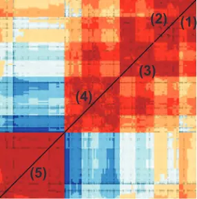
pa-rameter to the algorithms. Here, we use a more robust implemen-tation of k-means by utilizing a method called partitioning around medoids [Kaufman and Rousseeuw 2005]. One additional cluster formation solution we propose is to employ directly the tendency view to manually draw groups on the view’s diagonal. Our inten-tion here is not to replace clustering algorithms, but to allow for more precise cluster evaluation process. For instance, using the ten-dency view from Fig. 3 (left) we perform manual clustering where five groups are formed. We can clearly spot only cluster(5); while the upper clusters are not that clearly separable and requires further analysis (Fig. 4). All the clusterings, which are created manually, algorithmically or on different dimensions of the dataset become a part of the dataset itself at the end of this phase.

(1)

(2)

(3)

(4)

(5)

Figure 4: The interactive cluster formation using the tendency view and dissimilarity matrix. User draws a set of edges on the matrix diagonal, where each edge represents a cluster. This allows to create manual clusterings based on user priorities. Here, we specify five clusters that can be visually separated from each other.

3.3 Parallel Cluster View

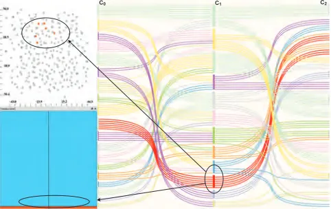
Clusters provide high level information about the internal structure of the data. In order to analyze the underlying relations in the data, we incorporate clusters as data dimensions in IVA operations. Ac-cordingly, we introduceParallel Cluster Views (cluster view) to ex-plicitly use clusters in brushing & linking operations. PCV, which is analogous to parallel sets proposed by Kosara et al. [Kosara et al. 2006], displays a number of different clusterings and enables the user to make selections at cluster level.

In a cluster view, vertical axes visualize different clusteringsCk,

wherekindicates the order of the clustering axis, i.e., for the left-most axis,k=0; and each curve between the axes represent a single data item,oi. All axes contain a set of clusters where each cluster

is represented by a different color. Curves between axiskandk+1 are colored with respect to the colors of the clusters they are mem-bers of inCk. This coloring schema improves the comprehension

of membership changes between different clusterings.

Ordering of the items in a cluster is crucial on the perception of changes in membership relations. The ordering for the curves are computed by considering the overlapping members betweenCkand

Ck+1. Firstly, the items are grouped into branches, where a branch

represents the itemsci∩cjwhereci∈Ck,cj∈Ck+1. Secondly, the

curves within a cluster are drawn regarding the cluster’s branches with the next clustering. Using this methodology, we make sure that items that share the same cluster inCkandCk+1never overlap

in between two neighboring clusterings.

Cluster view provides an intuitive mechanism to analyze and com-pare a number of different clusterings. For instance, Fig. 5a dis-plays three clusterings (C0,1,2) (formed using the weights wf1 =

wf2=1 andwf3=wf4=0, Fig. 4) which are: manual grouping (C0) performed in Fig. 4, k-means clustering withkparameter as 5

(C1) and a hierarchical clustering (C2). As hierarchical clustering

contains a set of levels, the appropriate level to use in the visualiza-tion is determined interactively by the analyst.

Cluster view is tightly integrated into interactive analysis cycle by cluster level brushes and linkage to the selection mechanism in all other views. The user can select any number of clusters using one ofSoperators. For instance, in Fig. 5b a cluster lever brush (b1), highlights the items (arrows) in the other linked views in a

(b ) (b )

1 2

C₀ C₁ C₂

(1) (1)

(1) (2)

(2)

(2) (3)

(3)

(3) (4)

(4)

(5) (5)

(b )1

(a) (b) (c)

Figure 5: a) Parallel cluster view showing three clusterings (C0,1,2), whereinC0andC1are composed of five clusters andC2of three clusters.

Curves represent the item membership relations within the clusterings. Note that clusters (5),(5) and (1) in sequential clusterings from left to right are identical. b) Cluster brush (b1) is used to select items representing members of cluster (4) in clustering (C0). Brushed items are also

highlighted in the accompanied scatter plot and the histogram that depicts a ratio of selected items per the specie. c) Combining selections on cluster and object level to analyze items of interest according to their cluster membership. Cluster brushb1and subsequent application of the

∪operator with the histogram brushb2reveals how brushed items are distributed in all clusterings (circles).

select cluster 4 and directly observe all the items, members of clus-ter 4, in the accompanying histogram and scatclus-ter plot. In the his-togram, ratio of species in selected items can be observed.

Moreover, brushes in other views are linked to the cluster view and can be combined with cluster level brushes. In Fig. 5c the cluster level brush (b1) is combined with histogram brush (b2) with the

∪operation, which selects additional items being members of the third specie.

4

Cluster Analysis Procedures

In the following, we describe cluster analysis procedures in clus-ter formation and clusclus-ter evaluation phases. Formation phase cludes assessment of cluster tendency, while evaluation phase in-volves cluster comparison, coherence and stability. These proce-dures are showcased in CIVA environment.

Cluster formation phase starts with the exploration of a data subset and/or dimensions suitable for clustering. Tendency view assists the analyst to evaluate the clustering tendency of the selection be-fore clustering. In Fig. 6a we see the tendency view of a selection which is suitable for clustering as it contains apparent structures in it. However in Fig. 6b, tendency view displays almost a random dis-tribution which would yield to a less successful clustering. These

(a) (b)

Figure 6: Two tendency views depicting different clustering ten-dencies. (a) contains apparent structure suitable for clustering. (b) is not preferable for clustering as no structure is easily visible.

views provide the reasoning to favor a specific selection and/or di-mension combination. Therefore, in this case (a) is preferred for clustering.

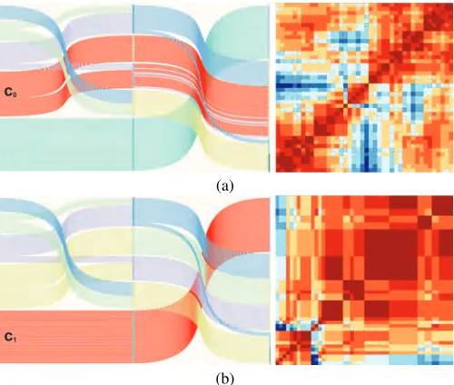
In the evaluation phase, clusters are visualized and compared to assess their meaning and validity . Evaluation of a cluster begins withcoherenceassessment. Tight cooperation between tendency view and cluster view in assessing cluster coherence can be seen in Fig. 7 where two cluster level brushes (to select clustersc0 and

c1) are visualized with their corresponding dissimilarity matrices.

Selected clusterc0results in a tendency view which depicts

sub-c0

(a)

c1

(b)

Figure 7: Two clusters (c0,1) and their corresponding cluster views.

Asc0contains apparent structures, it requires further refinement.

c1results in a uniform tendency view and it can be regarded as a

satisfactory cluster.

groups, which means it needs further refinement to get more valid results. However, tendency in the bottom row indicates that dis-tances between items inc1 are uniform, meaning that the cluster

con-centrate on finding better clusterings for the items inc0.

In cluster analysis, evaluatingcluster stabilityis a critical technique to validate clusters. In order to demonstrate cluster stability evalu-ation, we made several clusterings of the same selection using dif-ferentkparameters (k=3,7,10,15) for the k-means algorithm. If

the items in a certain cluster tend to stay in the same cluster ask

increases, this cluster can be considered as stable. Cluster labeled

c0 in Fig. 8 is a stable cluster as most of its members stay in the

same cluster in all the clusterings. On the other hand, members of

c

(a)

c

(b)

Figure 8: Using cluster views to evaluate cluster stability. Clus-ter view visualize four clusClus-terings made with k-means algorithm (k=3,7,10,15). Clusterc0is a stable cluster as most of its

mem-bers are in the same cluster in consecutive clusterings. Howeverc1

needs further refinement as its members are spread across different clusters in later results

c1 are spread among a number of different clusters withk=15.

Compared toc0,c1can be regarded as an unsatisfactory cluster as

there is an inconsistency between different runs of the clustering algorithm.

5

Case study:

cluster analysis of mixed

lipid bilayers

To demonstrate the usefulness of our approach, we present a study of cluster formations in lipid bilayers of biological membranes. Here, we do not focus on the cluster formation phase, but rather to showcase the importance of the evaluation phase. Our case study proved to be beneficial in getting better insight into data, which then led to new points of discussion on lipid bilayers. Biological membranes are active players in most biological processes and the dynamic behavior of the lipids which constitute them is decisive. In an attempt to understand biological membranes and membrane proteins, lipid bilayers have been and still are extensively stud-ied. Molecular dynamics (MD) simulations are utilized as powerful

tools to describe the atomic structure and dynamics of lipid bilay-ers, since detailed structural data of the most biologically relevant phases is difficult to obtain experimentally. In particular mixtures containing more than one lipid type have been studied in order to understand how different lipid types cluster together and can lead to inhomogeneity in biological membranes [Broemstrup and Reuter 2010]. Unfortunately, data generated by MD simulations can be rather tedious to analyze. Moreover, the analysis is nowadays per-formed on a non-interactive basis thus inactivating the user in the analysis of, e.g., cluster formation and cluster evaluation. In this study, we have found our framework to be highly beneficial for lipid clustering analysis of MD data.

The MD dataset of a mixed lipid bilayer [Broemstrup and Reuter 2010] is constituted of DMPC (dimirystoilphosphatidylcholine) and DMPG (dimirystoilphosphatidylglycerol) lipids. Each lipid is represented by one particle, localized at the position of the phos-phorus atom. The particles (items) undergo stochastic oscillation movements inxandydirections, and only slight variations along thezaxis, where the number of time steps in our simulation equals 1640. We extend the dimensionality of the dataset by computing the first derivatives of the movements,x′andy′. Additionally, the items have a regular variable representing their categories as mentioned above; i.e., DMPC and DMPG. The lipids are positioned in two separated layers along thezaxis and computational biologists are mostly interested in analyzing these lipid layers separately. There-fore, we limit our analysis to one of thez-layers by brushing the upperz-layer prior to the analysis.

To perform clustering on different time intervals, we brush the time intervals; [50,150],[700,800] and [1540,1640]. These intervals

were clustered separately using hierarchical clustering based onx

andycoordinates. We discovered groups of items, separated at the beginning, which form a cluster in the middle of the simulation and separate again at the end of the simulation. In Fig. 9 three ani-mated scatter plots are shown, which depict the distribution of such a group (c). These plots display the same items in thex−yplane

c

t0= 100 t1= 750 t2= 1600

Figure 9: Using the cluster view to compare clusterings per-formed in three distinct time intervals, [50,150],[700,800], and [1540,1640]. The analysis reveals a number of groups that are

sep-arate att0, cluster together att1and separate again att2. Animated

scatter plots justify this claim.

at different time steps (t0=100,t1=750,t2=1600). The scatter

plots visualize how two groups of items att0, form a single group

att1, and then separate into smaller groups again att2. This type of

lipid domains (rafts) in biological membranes. Moreover the abil-ity of interactively following the composition of the clusters has no equivalent in the non interactive methods for MD analysis.

In general, computational biologists cluster MD data using only theirxandycoordinates. However, in some cases it would be bene-ficial to form clusterings according to their velocities,x′andy′, and evaluate the results. The same set of lipids is clustered using three different weight distributionsw=

wx,wy,wx′,wy′

. ClusteringC0

is formed withw=h1,1,0,0i,C1withw=h1,1,1,1i, andC2with

w=h0,0,1,1i. In fig. 10, the first clustering is based solely on

C1

C0 C2

Figure 10: Using the cluster view to compare clusterings performed on different dimension subsets.C0is created on lipid positions,C2

on lipid velocities andC1on a combination of all these dimensions.

The selected cluster reveals a group of items which constitute a velocity cluster in addition to their positional cluster. Histogram displays lipid type distribution.

positions, the second one on a combination of positions and veloci-ties, and the third one only on velocities. This provides a very clear image on how much the clusterings differ in their positions with respect to their velocities. We can easily evaluate whether there is a correlation between these two types of clusterings by cluster se-lections. Notably, an interesting outcome of this analysis is when an equal number of DMPC and DMPG type lipids form a posi-tional cluster (fromC0), these items also have similar velocities.

On the other side, positional clusters containing an unequal number of different type of lipids do not have the same velocities. Fig. 10 displays one of the clusters discovered in the analysis, by utilizing the cluster view.

In one clustering procedure of lipid bilayers, we employed only the last 100 time steps from all 1640 frames to perform clustering analysis, due to the system stabilization [Broemstrup and Reuter 2010]. The clustering analysis pointed out a new issue that is to evaluate the influence of ’jumpers’ on the clustering process. Af-ter the visualization of the derivativesx′andy′, we found out that nearly half of all the items exhibit big ’jumps’ at a certain point of MD simulation. These jumpers correspond to atoms exiting at one side of the simulation bounding box and entering through the opposite one, which clamps the atoms along boundaries. Neverthe-less, usually all the simulated particles are employed for the cluster analysis. On one hand, the exploited clustering technique [Broem-strup and Reuter 2010] that is used to analyze the MD simulation, takes every time step separately. Therefore such particles do not have to be considered as outliers. On the other hand, when clus-tering is performed over a time interval, where dissimilarity matrix summation is involved, these jumpers can cause cluster instability when jumping from one cluster to another. Once clustering is done,

clusters are analyzed according to the distribution of their items’ categories; i.e., DMPC or DMPG.

We perform a hierarchical clustering wherein the jumpers were in-cluded. Consequently we have the possibility to evaluate the effect of jumpers on the clustering by means of the cluster view and other linked views (Fig. 11). In the figure, the clusterings represent 5

(b )

(b )₃

4

(b )₁

(b )₂

Figure 11: Discovery of jumpers within existing clusterings. The composed brush bL= (b1∪b2)∩b3 selects the jumpers that are

displayed in the animated scatter plot. The cluster view depicts their occurrence in individual clusterings. The cluster containing 4 jumpers was selected (bL∩b4) to reveal their position (arrows and

circles) within the cluster. The histogram depicts classification of the jumpers into DMPC and DMPG classes.

levels of a single hierarchical clustering (bottom left) performed on the last 100 time steps. The function graphs (top three right) are used to render derivativesx′andy′, where we employed brush

bL= (b1∪b2)∩b3to pick up the jumpers. The third function graph

delimits the selection only to the upper layer for 100 time steps (b3),

where all 1640 time steps are visible. For the better understanding of the particles’ movements we used an animated scatter plot (top left), where a user can directly observe the selected items in a fo-cus+context style in thex−yplane. The selection in the parallel cluster view reflects the occurrence of jumpers in individual hierar-chical levels. The jumpers participate more and more on clusterings as we increase the cluster level, where the lowest cluster represents non-clustered items. In the animated scatter plot we discover the relation of jumpers per individual cluster by makingbL∩b4

opera-tion in the cluster view, which displays the group of jumpers from the same cluster (arrows and circles, delimited byb4). As one can

clearly see, one of them has radically moved (left circle), while still being the member of the same cluster. Additionally, the his-togram (bottom right) depicts the classification of the jumpers into DMPC and DMPG classes. It can be deduced from the example that jumpers are not a crucial choice for the smaller clusters; how-ever when building bigger ones, their presence should be taken into account.

5.1 Implementation Details

tendency view. Therefore, the computation of these values is done in the GPU using CUDA. The resulting values are then transferred to the visualization pipeline through the GPU memory. This mech-anism ensures that the framework operates at interactive rates.

6

Conclusion

In this paper, we introduce a novel concept for visual cluster anal-ysis, which tightly integrates cluster formation and cluster evalu-ation, embedded within interactive visual analysis. In cluster for-mation we assist the users to explore subsets of the data that are suitable for clustering. In cluster evaluation, we utilize techniques from data mining to assess the cluster validity. These techniques are based on cluster comparison, cluster tendency, cluster coher-ence, and cluster stability, and they prove to be beneficial in order to achieve a successful cluster analysis in IVA. Consequently, the integration of these techniques leads to a better understanding of the underlying relations in the data.

The realization of our framework, CIVA, enriches the conventional interactive visual tools with two specific views capable of integrat-ing clusters into IVA. The cluster tendency view enables the evalua-tion of the current selecevalua-tion of items for possible clusterings. More-over, it allows the assessment of the cluster coherence in existing clusterings. The parallel cluster view provides a visualization of the item-to-cluster relationship, the evaluation of cluster stability and coherence, and importantly, the cluster comparison. The clus-ter view selection mechanism allows to link clusclus-ter level selections with selections made in conventional views.

We demonstrated CIVA in molecular dynamics simulations analy-sis, where the presented techniques leads to new considerations in the discussion on lipid bilayers. We performed three cluster anal-yses, where we studied the influence of velocities, time intervals, and ’jumpers’ on the simulation and its analysis.

As a future work, we will extend the scalability of the proposed views. Accordingly, in order to display few thousands of items in the tendency view, it is required to adapt the dissimilarity matrix appropriately. This can be achieved by displaying only a certain hi-erarchical level of dissimilarity matrix instead of the full resolution rows.

To conclude, with the proposed integration we managed to over-come the challenges that relate to the black-box nature of cluster-ing algorithms. Moreover, we believe that our framework provides more reliable clusterings and when integrated into IVA, these clus-terings provide even better insight into the underlying relations in the data.

7

Acknowledgements

NR acknowledges funding from the Bergen Research Foundation (BFS; Bergens Forskningstiftelse) and the University of Bergen. We thank Torben Broemstrup for molecular dynamics simulation data.

References

BEZDEK, J.,ANDHATHAWAY, R. 2002. Vat: a tool for visual assessment of (cluster) tendency. InNeural Networks, 2002., vol. 3, 2225 –2230.

BROEMSTRUP, T.,AND REUTER, N. 2010. Molecular Dynamics Simulations of Mixed Acidic/Zwitterionic Phospholipid Bilayers. Biophysical journal 99, 3 (Aug.), 825–833.

FISHER, R. A. 1936. The use of multiple measurements in taxonomic problems. Annals of Eugenics 7, 7, 179–188.

GROTTEL, S., REINA, G., VRABEC, J.,ANDERTL, T. 2007. Visual verification and analysis of cluster detection for molecular dynamics. IEEE Transactions on Visualization and Computer Graphics 13, 6, 1624–1631.

JAIN, A. 2010. Data clustering: 50 years beyond k-means.Pattern Recognition Letters 31, 8, 651–666.

KAUFMAN, L.,ANDROUSSEEUW, P. 2005.Finding Groups in Data: An Introduction to Cluster Analysis. Wiley’s Series in Probability and Statistics. John Wiley and Sons, New York.

KEIM, D., ANDRIENKO, G., FEKETE, J., G ¨ORG, C., KOHLHAMMER, J., AND

MELANC¸ON, G. 2008. Visual analytics: Definition, process, and challenges. In-formation Visualization, 154–175.

KONYHA, Z., MATKOVIC, K., GRACANIN, D., JELOVIC, M., ANDHAUSER, H. 2006. Interactive visual analysis of families of function graphs.IEEE transactions on Visualization and Computer Graphics 12, 6, 1373–1385.

KOSARA, R., BENDIX, F.,ANDHAUSER, H. 2006. Parallel sets: interactive explo-ration and visual analysis of categorical data.Visualization and Computer Graph-ics, IEEE Transactions on 12, 4, 558 –568.

LANGE, T., ROTH, V., BRAUN, M.,ANDBUHMANN, J. 2004. Stability-based validation of clustering solutions.Neural Computation 16, 6, 1299–1323.

LEX, A., STREIT, M., PARTL, C., KASHOFER, K.,ANDSCHMALSTIEG, D. 2010. Comparative analysis of multidimensional, quantitative data. Visualization and Computer Graphics, IEEE Transactions on 16, 6, 1027 –1035.

MARTIN, A. R.,ANDWARD, M. O. 1995. High dimensional brushing for interactive exploration of multivariate data. InVIS ’95: Proceedings of the 6th conference on Visualization ’95, IEEE Computer Society, Washington, DC, USA, 271.

RINZIVILLO, S., PEDRESCHI, D., NANNI, M., GIANNOTTI, F., ANDRIENKO, N.,

ANDANDRIENKO, G. 2008. Visually driven analysis of movement data by pro-gressive clustering.Information Visualization 7, 3, 225–239.

RUBEL, O., WEBER, G., HUANG, M.-Y., BETHEL, E., BIGGIN, M., FOWLKES, C., LUENGOHENDRIKS, C., KERANEN, S., EISEN, M., KNOWLES, D., MALIK, J., HAGEN, H.,ANDHAMANN, B. 2010. Integrating data clustering and visu-alization for the analysis of 3d gene expression data.Computational Biology and Bioinformatics, IEEE/ACM Transactions on 7, 1, 64 –79.

SCHRECK, T., BERNARD, J., TEKUSOVA, T.,ANDKOHLHAMMER, J. 2008. Vi-sual cluster analysis of trajectory data with interactive Kohonen Maps. InIEEE Symposium on Visual Analytics Science and Technology, 2008. VAST’08, 3–10.

SEO, J.,ANDSHNEIDERMAN, B. 2002. Interactively exploring hierarchical clustering results.IEEE Computer 35, 7, 80–86.

SHARKO, J., GRINSTEIN, G., MARX, K., ZHOU, J., CHENG, C.-H., ODELBERG, S.,ANDSIMON, H.-G. 2007. Heat map visualizations allow comparison of mul-tiple clustering results and evaluation of dataset quality: Application to microarray data. InInformation Visualization, 2007. IV ’07. 11th International Conference, 521 –526.

SHARKO, J., GRINSTEIN, G.,ANDMARX, K. 2008. Vectorized radviz and its appli-cation to multiple cluster datasets. IEEE transactions on Visualization and Com-puter Graphics, 1444–1427.

SHI, K., THEISEL, H., HAUSER, H., WEINKAUF, T., MATKOVIC, K., HEGE, H.,

ANDSEIDEL, H. 2009. Path line attributes-an information visualization approach to analyzing the dynamic behavior of 3d time-dependent flow fields. Topology-Based Methods in Visualization II, 75–88.

SIIRTOLA, H. 2004. Interactive cluster analysis. InIV ’04: Proceedings of the In-formation Visualisation, Eighth International Conference, IEEE Computer Society, Washington, DC, USA, 471–476.

SMITH, S.,ANDJAIN, A. 1984. Testing for uniformity in multidimensional data. IEEE transactions on pattern analysis and machine intelligence 6, 1, 73–81.

SPRENGER, T., BRUNELLA, R.,ANDGROSS, M. 2000. H-BLOB: a hierarchical visual clustering method using implicit surfaces.Proceedings Visualization 2000., 61–68,.

TAN, P., STEINBACH, M.,ANDKUMAR, V. 2006. Introduction to data mining. Pearson Addison Wesley Boston.