Hardware implementation algorithm and error analysis of high-speed fluorescence lifetime sensing systems using center-of-mass method

Hardware implementation algorithm and error analysis

of high-speed fluorescence lifetime sensing systems

using center-of-mass method

Day-Uei Li Bruce Rae

University of Edinburgh

Institute for Integrated Micro and Nano Systems共IMNS兲 School of Engineering

Faraday Building, The King’s Buildings Edinburgh EH9 3JL, Scotland

Robin Andrews University of Edinburgh School of Chemistry

Joseph Black Building, King’s Buildings Edinburgh EH9 3JJ, Scotland

Jochen Arlt

University of Edinburgh

School of Physics and Astronomy

Joseph Black Building, The King’s Buildings Edinburgh EH9 3JJ, Scotland

Robert Henderson University of Edinburgh

Institute for Integrated Micro and Nano Systems共IMNS兲 School of Engineering

Faraday Building, The King’s Buildings Edinburgh EH9 3JL, Scotland

Abstract. A new, simple, high-speed, and hardware-only integration-based fluorescence-lifetime-sensing algorithm using a center-of-mass method共CMM兲is proposed to implement lifetime calculations, and its signal-to-noise-ratio based on statistics theory is also deduced. Com-pared to the commonly used iterative least-squares method or the maximum-likelihood-estimation–based, general purpose fluorescence lifetime imaging microscopy 共FLIM兲 analysis software, the proposed hardware lifetime calculation algorithm with CMM offers direct cal-culation of fluorescence lifetime based on the collected photon counts and timing information provided by in-pixel circuitry and therefore delivers faster analysis for real-time applications, such as clinical diagnosis. A real-time hardware implementation of this CMM FLIM algorithm suitable for a single-photon avalanche diode array in CMOS imaging technology is now proposed for implementation on field-programmable gate array. The performance of the proposed methods has been tested on Fluorescein, Coumarin 6, and 1,8-anilinonaphthalenesulfonate in water/methanol mixture. ©2010 Society of Photo-Optical Instrumentation Engineers. 关DOI: 10.1117/1.3309737兴

Keywords: lifebased sensing; fluorescence lifetime imaging microscopy; time-resolved imaging; photon counting; single-photon avalanche diode; center-of-mass.

Paper 09371R received Aug. 21, 2009; revised manuscript received Nov. 14, 2009; accepted for publication Dec. 2, 2009; published online Feb. 16, 2010; corrected Feb. 23, 2010; corrected Mar. 2, 2010.

1 Introduction

Time-resolved fluorescence lifetime imaging 共FLIM兲 is widely used in cell-biology research, medical diagnosis, and pharmacological development.1–3It is based on the measure-ment of the decay in fluorescence emission across a sample after optical excitation and can be used to quantify physi-ological parameters, such as pH,Ca2+_,pO

2, etc., in biological samples. The independence of fluorescence lifetimes from probe concentration makes FLIM more favored than its counterpart—fluorescence intensity imaging. As shown in Fig. 1共a兲, a laboratory FLIM experiment usually contains a Ti-sapphire laser, a photomultiplier tube 共PMT兲, a time-correlated single-photon counting 共TCSPC兲 photon-counting card, fluorescence lifetime analysis software, and a PC graphi-cal user interface共GUI兲. Available FLIM systems provide ex-cellent time resolution and light sensitivity, although they are quite expensive and cumbersome. Commercial applications increasingly demand compact and portable system-on-chip

共SOC兲FLIM solutions. Thanks to the progress of semicon-ductor technology, high-accuracy time resolution, high sensi-tivity, low cost, and compactness can be achieved by

exploit-ing CMOS sexploit-ingle-photon avalanche diode共SPAD兲arrays with low dark count rate to replace PMTs4–7and by bump-bonding AlInGaN UV micropixellated light-emitting diodes to replace lasers7in the general direction of lab on chip. The imager can include a CMOS SPAD array with in-pixel digital counters or time-to-digital converters共TDCs兲6,7that allows recording not just the photon counts but also the raw timing data for de-tailed scientific analysis. The imager also contains Field-programmable gate arrays共FPGAs兲allowing data processing. Figure1共b兲shows the SOC solution suited to lab-on-chip ap-plications, which is intended to replace the system of Fig. 1共a兲. For imaging purposes, a remaining challenge is that the excessive computational demands of available lifetime analy-sis software such as the iterative least-squares method共LSM兲 or maximum-likelihood-estimation 共MLE兲8 render real-time imaging impossible. A new FLIM algorithm considering the instrument response based on the Laguerre expansion technique9speeds up lifetime calculations, but the computa-tion time increases with imager size. However, in many ap-plications, such as microfluidic mixing10and exploratory bio-logical experiments, it is desirable to monitor the instantaneous biochemical interactions to provide quick feed-back to corresponding manipulations. The slow speed of LSM- or MLE-based software analysis tools becomes a

1083-3668/2010/15共1兲/017006/10/$25.00 © 2010 SPIE Address all correspondence to: Day-Uei Li, University of Edinburgh, Institute for

bottleneck and has driven the recent development of nonitera-tive, compact, and fast real-time time-domain FLIM systems11–17 and real-time frequency-domain FLIM algo-rithms and systems.18–21In the past, rapid lifetime determina-tion methods 共RLD兲 were thought to be the simplest algorithms11 and were used in some previously reported video-rate FLIMs.12,13 In Ref. 12, an optomechanical delay control for RLD was proposed; however, its cumbersome op-tical setup makes it difficult to image a wide range of fluoro-phore lifetimes, and an electronically controllable delay would be preferable.13 To further achieve compactness for SOC, we can exploit configurable devices such as FPGAs to realize real-time FLIM systems. FPGAs have significantly benefited from the advances of CMOS technology. The latest FPGAs contain over hundreds of millions of transistors and can easily accommodate the output signals from SPAD arrays of growing size. With the ability of configuration, designers can easily reconfigure FPGAs by hardware description lan-guage to perform any application-specific logic functions, such as real-time lifetime calculations. We therefore evaluated the possibility of applying RLD either on chip or on FPGA and concluded that RLD can be implemented on FPGA with lookup tables共LUT兲 of natural logarithmic14 or other func-tions if overlap gating techniques are used.14,15The delay con-trol of RLD can be easily reconfigured by users, and we ex-pect that the system can benefit greatly from the user-friendly features. However, building a LUT on FPGA covering a wide range of lifetimes is inefficient, and it is desirable to develop more FPGA-friendly algorithms that use only additions. The impact will be huge, especially when a large SPAD array is applied. Moreover, a major drawback of RLD is the require-ment to choose a proper time delay between two time gates,11–14which is quite challenging when specimens with a wide range of lifetimes coexist. We therefore propose a more hardware-friendly algorithm for lifetime calculations based on the imager developed in Ref.6. In this paper, we first intro-duce the proposed hardware lifetime calculation algorithm by considering a single-exponential decay for simplicity. Al-though it is possible to implement multiexponential algo-rithms in hardware in combination with software calculations,17 it is not economic in terms of hardware re-sources. The single-exponential assumption allows a proper

comparison of various fitting algorithms. Moreover, a single-exponential decay model is still useful to contrast different types of fluorophores. For diagnostic applications, obtaining lifetime contrast is probably more important than calculating the absolute values of lifetimes.13The FPGA implementation and Verilog/Matlab modeling of the center-of-mass 共CM兲 method 共CMM兲will be introduced. The performance of the proposed algorithm will be tested using Fluorescein, Cou-marin 6, and 1,8-anilinonaphthalenesulfonate共ANS兲in water/ methanol.

2 Theory

2.1 CM of a Single-Exponential Function

For an object with a continuous distribution of mass density

f共r兲and total massMT, its CM is defined as

CM⬅

冕

rf共r兲dV

冕

f共r兲dV

=

冕

rf共r兲dV

MT

. 共1兲

For a mass density of a single-exponential function f共t兲=A

exp共−t/␶兲in the range0艋t艋T, we have

冕

0 T

tf共t兲dt=

冕

0

T

Atexp共−t/␶兲dt=A␶2_{共1 − e}−T/␶_兲−A␶Te−T/␶

=␶

冕

0 T

f共t兲dt−A␶Te−T/␶_, TCSPC

Card

Titanium-Sapphire Laser

Real-time

Image

Fast FLIM Algorithms

CMM FPGA PC and Software Tools for

Fluorescence Lifetime Analysis PMT

Sample

Sample LED

Array [7]

Chip SPAD Array [5,6] LED

Drivers

TDC

Digital Readout Bump Bond

(a) (b)

Fig. 1 共a兲Laboratory FLIM and共b兲FLIM system on chip.

0 CM t T

0 A

(a) f(t) f(t) = Aexp(−t/τ)

t

0 t1 t2 t3 tM−1 tM

(b) τ

0 A

f(

t)

N

0 N

1 N

2 _{. . .}

N

M−1

f(t) = Aexp(−t/τ)

t_j+1− t_j= h j = 0, 1, 2, .., M−1 f(t₀)

f(t

1)

f(t

2)

f(t

3)

f(t

M−1)f(t

M)

[image:2.630.363.531.71.268.2] [image:2.630.72.299.72.231.2]

⇒CM =

冕

0 T

tf共t兲dt

冕

0 T

f共t兲dt

=␶− Te −T/␶

1 − e−T/␶. 共2兲

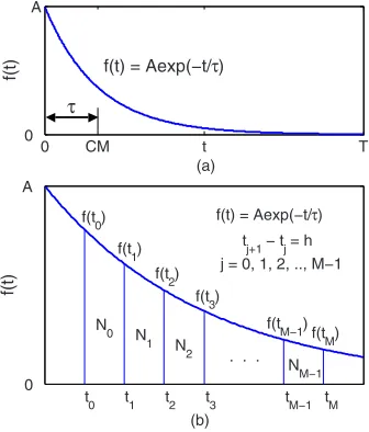
AsT⬎7␶, the center of mass lies at the position with a dis-tance of␶from the origin as Fig.2共a兲shows. Iff共t兲represents a fluorescence histogram, then the denominator of Eq.共2兲will be the total photon count, while the numerator is the sum of temporal information of total photon events. To implement Eq.共2兲in hardware, denoted as CMM for simplicity, we need to quantize the temporal information by dividing the measure-ment window intoM time bins共bin width ofh兲, as shown in Fig. 2共b兲, using TDCs in the photon counting module. An interesting analog circuit was proposed to calculate Eq.共2兲for single-molecule microscopy;16 however, it did not describe how to remove background noise in the analog domain. In such applications with low fluorescence emission, background-to-signal ratio will be relatively significant. Com-pared to Ref.16, CMM works in the digital domain and al-lows background noise to be removed much more easily.

2.2 Error Analysis of CMM

In Ref.22, it was shown that Eq. 共2兲is equivalent to MLE when M→⬁; therefore, CMM can be viewed as hardware version of MLE. When the ratio of the full width at half maximum 共FWHM兲 of the instrumental response function

共IRF兲over the lifetime isⰆ1, we can assume the fluorescence decay histogram f共t兲=A exp共−t/␶兲 with ␶ being the lifetime.17 For the usual measurement setup in a lab, the FWHM of the IRF is on the order of hundreds of picoseconds; thus, it is reasonable to target lifetimes of⬎500 ps. With the assumption of single-exponential decay, the lifetime␶ is re-lated to the decay function as

␶⬵

冕

⌬tf共t兲dt

冕

f共t兲dt

=

冕

t0

t₁

共t−t0兲f共t兲dt+_¯+

冕

t_M−1 t_M

共t−t0兲f共t兲dt

冕

t₀ t_M

f共t兲dt

⬵

冕

t0

t₁

冉

t₀+t₁

2 −t0

冊

f共t兲dt+¯+

冕

_t M−1

t_M

冉

tM−1+tM

2 −t0

冊

f共t兲dt

冕

t0

tM

Aexp共−t/␶兲dt

=

兺

_j=0

M−1

⌬tj

冕

tj

t_j+1

f共t兲dt

N_c =

兺

_j=0

M−1

⌬tjNj

N_c =

Nc 2 +

兺

_j=0

M−1

jNj

N_c h

=

冢

兺

_j=0

M−1

jNj

N_c +

1

2

冣

h=Rh, 共3兲

where ⌬tj=tj−t0+h/2 =共j+ 1 − 1/2兲h and Nj is the number of recorded counts in thej’th time bin共j= 0, 1,…,M− 1兲, and

N_c=A␶关1 − exp共−Mh/␶兲兴 is the total effective signal count. The recorded variablesNj are independently Poisson

distrib-uted with respective mean valueENj=兰jh

共j+1兲h_f共t兲dt

and stan-dard deviation␴Nj=共ENj兲1/2, and we thus have

Nj=ENj+␴Nj=Ncxj共1 −x兲共1 −xM兲−1+␴Nj, 共4兲

where x= exp共−h/␶兲. Substituting Eq. 共4兲 into Eq. 共3兲, we have

␶CMM⬵

兺

_j=0 M−1

⌬tj共ENj+␴Nj兲

兺

_j=0 M−1

共ENj+␴Nj兲 =

兺

_j=0 M−1

⌬tjENj+

兺

j=0 M−1

⌬tj␴Nj

兺

_j=0 M−1

ENj+

兺

j=0 M−1

␴Nj

=U+␴u

V+␴v=

U V

1 +␴u/U

1 +␴v/V =␶

冉

1 + ⌬␶

␶

冊冉

1 + ␴u

U − ␴v

V

冊

, 共5兲 where

U=

兺

j=0 M−1

⌬t_jEN_j, V=N_c, ␴u=

兺

j=0 M−1

⌬t_j␴N_j,

␴v=

兺

j=0 M−1

␴Nj. 共6兲

From Eqs.共4兲and共6兲, we have

U V=

h共1 −x兲

1 −xM

兺

_j=0

M−1

冉

j+ 1 −1 2

冊

x

j₌h共1 −x兲

1 −xM 共x+ ¯+x

M_兲⬘−h 2

=h

冋

1 −共M+ 1兲x

M_+MxM+1

共1 −x兲共1 −xM兲 −

1

2

册

=hG共x兲=␶

冉

1 +

⌬␶ ␶

冊

;

therefore, we have the accuracy equation

⇒⌬␶CMM

␶CMM =h

␶G共x兲− 1, 共7兲

G共x兲=1 +x−共2M+ 1兲x

M_{+共2M− 1兲x}M+1

2共1 −x兲共1 −xM兲 . 共8兲

From Eqs.共5兲–共7兲, we have the precision equation

␴␶CMM

␶CMM

=

冉

1 +⌬␶

␶

冊冉

␴u

U − ␴v

V

冊

= h ␶G共x兲

冉

␴u U −

␴v

V

冊

, 共9兲

␴u U −

␴v

V =

冑

兺

_j=0

M−1

冋

冉

⌬tj

U −

1

Nc

冊

2

␴N_j2

册

=

_冑

1

NcG共x兲

冑

冉

1 −x

1 −xM

冊

兺

_j=0

M−1

冋

j+1

2−G共x兲

册

2

xj

=

_冑

1

Nc

冑

P共x兲

P共x兲=x−M2xM+共2M2− 2兲xM+1−M2xM+2+x2M+1.

共11兲 The accuracy of the CMM lifetime estimator is determined by the quantization error in Eq. 共3兲. It is usually predictable and can be calibrated by software,17 whereas the precision

共normalized standard deviation兲mainly comes from Poisson noise and can be improved only through increasing photon count. From Eqs. 共2兲and共3兲, we can also calibrate the life-time by

␶CMM,Cal⬵␶CMM+

Te−Mh/␶CMM 1 − e−Mh/␶_CMM=

冉

R+

Me−M/R 1 − e−M/R

冊

h.

共12兲 This calibration can be easily done by software and can im-prove the accuracy further toT⬎4␶.

Figure3shows the inverse accuracy and precision curves of Eqs.共7兲and共9兲共for easily transferred to decibels兲for M

= 1024 andNc= 217. The theoretical results marked as solid lines are compared to Monte Carlo simulations marked with crosses, giving good agreement and proving the correctness of Eqs. 共7兲 and 共9兲. Theoretical precision curves of 1024-bin MLE, and 2-gate RLD 共with gate widthwg=Mh/2 = 512h兲 are also provided for comparison. From Fig. 3, the optimal window for RLD is fromMh/␶= 1 – 5, whereas that for CMM is fromMh/␶= 7 – 100. Here, we define a new precision value for CMM as

Precision⬅ ␶CMM

冑

␴␶CMM 2 _+⌬␶

CMM

2 . 共13兲

In applications, there is no need to define this new precision as long as the accuracy can be enhanced by software calibra-tion as described above. For simplicity, we assume there is no software calibration available. The new precision definition

facilitates end users to familiarize themselves with the sensing system and easily choose a proper parameter. The new preci-sion curve is also shown in Fig.3. Its optimal window is the same as that of MLE fromMh/␶= 10– 100.

In some applications, we need to know the range of life-times that a predictor can resolve when the laser repetition rate共LPR兲 or the measurement window 共MW兲 is fixed. We use theFvalue introduced in Ref.23to quantify the perfor-mance of a lifetime imaging technique. TheFvalue is defined as F=N_c1/2␴␶/␶, where ␴␶ is the standard deviation of re-peated measurements of the lifetime value␶. Figure4shows

F curves for 1024-bin CMM, 4096-bin CMM, 1024-bin MLE, 15-bin integration for extraction method 共IEM兲,17and 2-gate RLD in terms of ␶normalized by measurement win-dow共MW=Mh兲. The MLE demonstrates the best resolvabil-ity range. However, it is not possible to implement it in hard-ware. For the other three methods, only CMM has a flat optimalFresponse. TakingLPR= 5 MHz as an example and assuming the TDC full range is equivalent to the measurement window, MW= 200 ns. If N_c= 217_{, then the lifetime range} with a precision of 40 dB 共F⬃4兲 for 2-gate RLD, 15-bin IEM, 1024-bin CMM, and 1024-bin MLE are 16–200, 12– 140, 0.6–30, and 0.02– 320 ns, respectively. For RLD, the optimal window can be chosen by selecting proper delays, mechanically or electronically.12,13 For CMM and IEM, the optimal window can be easily set on FPGA by choosing a properM. In theory, the lower bound of CMM and MLE can be further reduced by increasingM. However, it is limited by the FWHM of the system IRF, which can be several hundreds of picoseconds, considering jitter contributed by the SPADs, laser, and TDCs. Therefore, increasing M further for real-time, single-exponential lifetime estimation is not sensible. A comparison summary for the CMM, IEM, RLD, and the MLE algorithms is provided in Table1. It clearly shows the merits of the CMM in terms of F value, lifetime resolvability, and on-chip feasibility. From Fig.4, the advantage of CMM is that its photon collecting efficiency, for a given precision, is 2.5-0 10 20 30 40 50 60 70

100 101 102 103 104 105

Measurement window M×h (τ): M = 1024

τ

/

στ

,

τ

/

∆τ

τ_CMM/∆τ_CMM

τ_CMM/στ_CMM

τ_RLD/στ RLD

τ_MLE/στ MLE

τ_CMM/(στ2_CMM+∆τ2_CMM)0.5

Fig. 3 Inverse precision and accuracy curves for the 1024-bin CMM, 1024-bin MLE, and 2-gate RLD withNc= 217共measurement window =Mh= 2wg兲.

10−3 10−2 10−1 100

1 2 3 4

τ/MW

F=(

στ

/

τ

)N

c

0

.5

MLE−1024 RLD

IEM−15 [17]

CMM−1024

CMM−4096

[image:4.630.71.299.70.284.2] [image:4.630.332.563.72.274.2]

fold larger than RLD-2 and IEM. The measurement window should be about10⫻the lifetime共or7⫻ with software cali-bration兲 to achieve high sensitivity共good photon economy兲. In this respect, RLD imaging can use a higher laser repetition rate and achieve a better duty cycle at measurement window= 1 – 5␶. However, if complete raw arrival time data are needed, the laser repetition rate cannot be too low. More-over, for most fluorophores, the measurement window is⬎4␶ to avoid nonidealities such as bleed through. Although one might argue that for mono-exponential decays the bleed through does not matter too much, but it undermines back-ground correction. This means our CMM detector system has a slightly lower duty-cycle performance in order to maintain the sensitivity. However, our system contains TDCs and can provide both raw data and lifetime data output.

2.3 Error Analysis of CMM with Background Correction

In most practical lifetime analysis tools, background is taken into account by the subtraction of a dc background valueC0

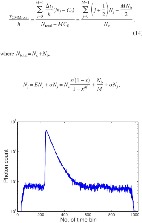
共=Nb/M,Nbis total background noise within a measurement window ofMh兲from the measured histogram, and along with lifetime calculations, this is done by software. However, for faster real-time imaging it is desirable that a hardware cali-bration technique can be integrated into the system by gener-ating the required C0 using the available counts. Figure 5 shows a typical measured histogram 共of1 ␮M Fluorescein, detailed in Section 4兲. There always exists a flat response before the peak of the histogram decided by the delay be-tween systems enable signal and laser excitation. A dc value ofC0can be obtained by averaging the counts of several bins on the flat response. Suppose we have a white background noise response, and we can therefore obtain the background count asNb=MC0, from Eq.共5兲, and by subtractingC0from the count in each bin, we have

␶CMM,corr

h =

兺

_j=0 M−1

⌬tj

h 共Nj−C0兲 N_total−MC₀ =

兺

_j=0 M−1

冉

j+1 2

冊

Nj−

MNb 2

N_c ,

共14兲

whereNtotal=Nc+Nb,

Nj=ENj+␴Nj=Nc

xj_{共1 −x兲} 1 −xM +

Nb

M +␴Nj, Table1 Comparison summary of the CMM, IEM, RLD, and MLE.

Method

Fmin

ath共␶兲 resolvabilityF⬍4

On-chip feasibility

Standard RLD-2

1.5 at 2.5

0.08⬍␶/MW⬍1 Yes/LUTb

IEM w/o

Calibration17

1.6

at 0.67a 0.06⬍_for␶/MW_M=15⬍0.7 Yes

IEM with

Calibration17

1.2 at 1.67

0.03⬍␶/MW⬍0.7

forM=15

Yes

MLE

M=1024

1.0

at关0.01–0.5兴 1⫻10

−4_{⬍␶/MW⬍1.6 No}

CMM

M=1024

1.0

at关0.01–0.1兴 3⫻10

−3_{⬍␶/MW⬍0.15 Yes}

CMM

M=4096

1.0

at关0.003–0.08兴 7⫻10

−4_{⬍␶/MW⬍0.15 Yes}

a_{The optimalhof IEM is independent ofM.} b_{On a small detector array.}

0 200 400 600 800 1000

101 102 103 104

No. of time bin

Ph

oton

count

[image:5.630.135.497.84.307.2] [image:5.630.327.565.352.725.2]

ENj=

冕

jh

共j+1兲h

关f共t兲+Nb/共Mh兲兴dt, and ␴Nj=共ENj兲1/2.

共15兲

The error equations can be obtained by replacing Eq.共15兲into Eq.共14兲and following the same procedure as Eqs.共4兲–共11兲.

3 Hardware Implementation Method and

Modeling

3.1 FPGA Implementation Method

We rewrite Eq.共3兲as

␶CMM

h =

兺

_i=1Nc D¯i

Nc +1

2, 共16兲

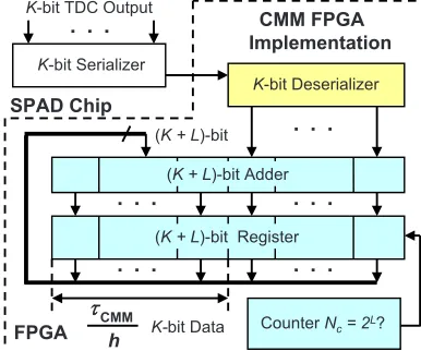
whereD¯iis theK-bit TDC output of thei’th captured photon. It is quite easy to implement Eq.共16兲on FPGA. It can also be readily modified to implement background correction of Eq. 共14兲. For simplicity, we introduce the FPGA implementation of Eq.共16兲. The first term on the right-hand side can be imple-mented by an adder for the numerator and a counter for the denominator. In Fig.6, a共K+ log2Nc兲-bit register is used to store the results from the adder and sends them back to the adder for adding with the TDC code of the next photon. The lifetime can be updated by latching the results when the counter storingNcreaches a value of

Nc= 2L, L is an integer. 共17兲

When this condition is reached, a trigger signal is sent to latch the latest ␶CMM/h and reset the register to perform the next calculation and keep updating the lifetime. By this arrange-ment, we do not even need digital division by only taking the firstKmost significant bit共MSB兲bits of the register or more thanKMSB bits for decimal accuracy. The second term1/2 on the right-hand side can be kept in mind or simply merging Eqs.共16兲and共17兲as

␶CMM

h =

兺

_i=1Nc D¯i+ 2L−1

2L , 共18兲

with only a minor effort on the FGPA resource because it is a global correction term for the whole SPAD array. From the discussion above, in the optimal window or lifetime resolving range for CMM, we have

F=Nc 1/2_␴␶

␶ =

2L/2_␴␶

␶ = 1.0⇒ ␶ ␴␶= 2L/2

or signal-to-noise ratio共SNR兲 ⬵3L共dB兲. 共19兲

This is a very convenient formula for end users. By selecting a proper L via the GUI, one can easily set the accuracy of images. For example, if a precision of SNR= 30 dB 共␴␶/␶ = 3%兲 is required for the system, the total count within the measurement window is2SNR/3_{= 1024. The expression of Eq.} 共19兲is the same with that of MLE in the optimal range. For imaging purposes, CMM can be applied to a column of SPAD pixels, and the hardware implementation can be extended ac-cordingly. For video-rate applications, we have to keep the lifetime update time to

tupdate= 2L

PCR艋30 ms, 共20兲

where PCR is the photon count rate. For example, for a pre-cision ofSNR= 30 dB with a lifetime update rate of⬎33 fps, the PCR should be larger than33 kHz, which is not a difficult task at all for the latest CMOS SPAD detectors.4–7End users can choose a proper L to maintain an acceptable accuracy while keeping the lifetime update rate. All parameters can be set by end users via the GUI considering the image contrast, accuracy, and update speed. Other functions, such as auto-matic histogram peak finding, imaging filtering, dark area marking, homogeneous lifetime updating, and background correction, can also be implemented on a FPGA. With this arrangement, video-rate lifetime images can be generated and the dynamics of interactions between fluorophores and the microenvironment, such as microfluidic mixing, can be easily observed.

3.2 SPAD Detection Model and Verilog/Matlab Simulations

Before employing CMM with a SPAD array, we first built a detection model of a SPAD pixel in order to verify the effi-ciency of the algorithm on the FPGA. Figure 7 shows the diagram for the detection model of a SPAD pixel. The8-bit signal coming from a TDC in a SPAD pixel cell can be mod-eled by a31-bit pseudo-random bit sequence共PRBS兲 genera-tor and a lookup table used for generating a photon-emission probability function. The threshold valuesVth,jare related as

Vth,j+1−Vth,j⬀Nj, j= 0, . . . ,M− 1. 共21兲 The overall jitter of the SPAD and laser共assumed as a Gauss-ian distribution兲, and the laser excitation delay between the electrical excitation signal and laser pulse is built right after the exponential lookup table. The SPAD detection model then

K-bit Deserializer

K-bit Serializer

K-bit TDC Output

CMM FPGA Implementation

CounterNc= 2L?

. . .

. . .

. . .

. . .

. . .

. . .

(K + L)-bit Register

SPAD Chip

FPGA

(K + L)-bit

K-bit Data

h

ττ

CMM

(K + L)-bit Adder

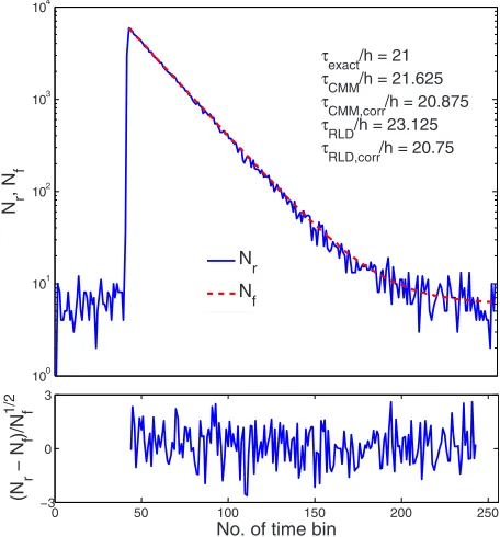
[image:6.630.86.279.72.233.2]

feeds the output data into a serializer to model the signal coming from the SPAD pixel and then via a deserializer to the CMM lifetime calculation module in Fig.6. The polynomial for generating the 31-bit PRBS is g共x兲= 1 +x28_+x31_.24 _The maximum length of the bit sequence is 231_{− 1 = 2.15⫻10}9_, which is much larger than the total photon count of usual TCSPC measurements for a single pixel. For comparison to RLD algorithms and for simplicity, we built a lookup table of digital division inside the CMM implementation block; al-though in practice, there is no need to do so according to Eqs. 共16兲 and 共17兲. Taking a single decay function f共t兲 =Aexp关−t/共21h兲兴 as an example, if h is of200 ps共the full range of the TDC is256h= 51.2 ns, which is equivalent to a LPR= 20 MHz兲. The lifetime ␶= 21h= 4.2 ns is much larger than a typical jitter of 300 ps such that only tail fitting is applied to extract the lifetime without digital deconvolution.17 A measurement window ofM= 200 共44th to 243rd bin兲from the peak of the histogram is chosen for lifetime calculations. Figure8shows the decay histogramNrobtained by the model and the fitted curveNfby CMM with background correction of Eq.共14兲using Verilog. The calculated lifetimes with four extra bits for decimal accuracy obtained by CMM and RLD with/without background correction are listed, respectively. The reduced chi-squared is 1.10 showing a good fit, and Fig. 8 also shows the normalized residual plot of共N_r−Nf兲/Nf

1/2_, which is well distributed, implying that the model is Poisson distributed as in real cases.

The second example is f共t兲=Aexp关−t/共2h兲兴, with a life-time ␶= 2h= 400 ps at LPR= 20 MHz. We are comparing CMM to other algorithms withM= 200. CMM is not sensi-tive to the timing jitter. For RLD, it is a challenging task to resolve lifetimes, much less than the effective measurement window共␶Ⰶ200h in this case兲. Thus, we use MLE8instead to calculate the lifetime with software using

1 +共x−1− 1兲−1−M共x−M− 1兲−1=Nc −1

兺

j=0 M−1

共j+ 1兲Nj, 共22兲

wherex= exp共−h/␶兲. In this example, all algorithms are per-formed on the computer for a fair comparison, and therefore, there is no digital quantization error for CMM. The reduced chi-squared is 0.94, and Fig.9shows the decay histogram and residual obtained by the model and the fitted curve by CMM with background correction using Matlab. The calculated

life-times for CMM and MLE are also listed. For CMM and MLE, it is necessary to apply background correction when resolving lifetime much less than the measurement window. It is also interesting to note that the behavior of CMM and MLE are almost identical in terms of precision and sensitivity to back-ground noise in the optimal lifetime range; therefore, CMM can be viewed as a hardware implementation algorithm of

31-bit Pseudo Random Number Generator Seed

CLK

31 8

Y

SPAD Detection Model

8 8

Y

TDC Output Exponential Function

Look-up Table

V_th0

Vth1 Vth2

Vth256 1

2 3

4

254 255 256

Jitter

Fig. 7 SPAD detection model implemented on FPGA.

0 50 100 150 200 250 −3

0 3

No. of time bin

(N

r

−N

f

)/N

f

1/2

100 101 102 103 104

N r

,

N f

τ_exact/h = 21

τ_CMM/h = 21.625

τ_CMM,corr/h = 20.875

τ_RLD/h = 23.125

τ_RLD,corr/h = 20.75

N r N

f

Fig. 8 Decay and fitted curves obtained by the model and CMM using Verilog.

0 50 100 150 200 250

−3 0 3

No. of time bin

(N

r

−N

f

)/N

f

1/2

100 101 102 103 104 105

N r

,

N f

τ_exact/h = 2

τ_CMM/h = 5.09

τ_CMM,corr/h = 1.97

τ_MLE/h = 5.12

τ_MLE,corr/h = 1.95

N r N

f

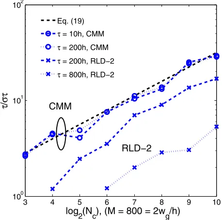
[image:7.630.91.281.72.204.2] [image:7.630.333.561.73.318.2] [image:7.630.332.564.473.724.2]

MLE although their physical definitions are not the same. Figure10 shows inverse precision curves versus total count for 800-bin CMM and 2-gate RLD 共2wg= 800h= 1␶ or 4␶兲 with Monte Carlo simulations for different lifetimes. CMM displays its uniform performance and higher photon-counting efficiency over a wide range of lifetimes. Therefore, CMM is suitable for low light detection.

4 Experimental Results

4.1 Measurements of Fluorescein and Coumarin 6 Using SPADs

Measurements of the decays of Fluorescein and Coumarin 6 mounted on microcavity slides have been made to test the proposed CMM hardware lifetime calculation algorithm. Table2 lists the fluorophores under test in terms of solvent, concentration, excitation and emission wavelengths, typical lifetimes provided by the manufacturers, and the calculated lifetimes using CMM, MLE, RLD-2, and Edinburgh Instru-ments F900 software. Then,45␮L of each sample was pipet-ted into a single-cavity共15-mm diam兲glass microscope slide

共Fisher Scientific, United Kingdom, MNK-140-010A兲 and sealed with a 0.12-mm-thick borosilicate glass coverslip

共Fisher Scientific, MNJ-300-020T兲. The LPR 共PicoQuant pulsed diode laser with wavelength of470 nm兲is 10 MHz, and the average output power is0.12 mW. Fluorescence de-cay curves were recorded on a time scale of100 ns, resolved into 1024 time bins 共i.e., h⬃0.098 ns兲. With LPR of 10 MHz, there is no bleed through observed on measured histograms. The fluorescence emission is captured by a SPAD array fabricated in a 0.35-␮m CMOS high-voltage process mounted on a daughter board. Figure5 shows the measured histogram of Fluorescein, and Fig.11shows the logarithmic plot for the measured histogramNr, starting from the bin with the peak intensity and the fitted curveNfby CMM with back-ground correction, and also the normalized residual count. The reduced chi-squared is 1.40. The last three rows of Table 2 show the calculated lifetimes with background correction for CMM, MLE, RLD, and Edinburgh Instruments F900 soft-ware, respectively. Measurement windows of 5 – 20/30␶,

3 4 5 6 7 8 9 10

100 101 102

log

2(Nc), (M = 800 = 2wg/h)

τ

/

στ

CMM

RLD−2

Eq. (19)

τ= 10h, CMM

τ= 200h, CMM

τ= 200h, RLD−2

[image:8.630.70.299.72.299.2]

τ= 800h, RLD−2

Fig. 10 Inverse precision curves versus total count of 800-bin CMM and 2-gate RLD for different lifetimes.

Table2 Summary of fluorophores used.

Fluorophore Fluorescein Coumarin 6

Solvent Ethanol Methanol

Concentration共␮M兲 1 1

Excitation wavelength共nm兲 495 460

Peak emission wavelength共nm兲 517 505

Typical lifetime共ns兲 4.1 2.5

Calculated lifetime共ns兲 using CMM

h=0.098 ns

4.15±0.15

5␶⬍Mh⬍20␶a _5␶2.42_⬍Mh⬍±0.08_30␶b

Calculated lifetime共ns兲 using MLE

h=0.098 ns

4.2±0.20

0.5␶⬍Mh⬍20␶ 0.5␶2.4⬍Mh⬍±0.130␶

Calculated lifetime共ns兲 using RLD-2 1␶⬍2wg⬍5␶

4.4±0.08 2.42±0.05

Calculated lifetime共ns兲using Edinburgh instruments F900

h=0.098 ns

4.38±0.06

1␶⬍Mh⬍20␶ 12.41␶⬍Mh±0.03⬍30␶

[image:8.630.140.498.463.734.2]

0.5– 20/30␶, 1 – 5␶, and 1 – 20/30␶ are chosen for CMM, MLE, RLD-2, and F900, respectively. The mean lifetimes of Fluorescein and Coumarin 6 calculated by CMM, are 4.15 and 2.42 ns, respectively, in good agreement with the data provided by the manufacturers and are also comparable to other algorithms.

4.2 Measurements of ANS in Water/Methanol Using PMTs

Fluorescent dye ANS is widely used in biological experiments due to its extreme sensitivity to the composition of water/ methanol mixtures, showing a drastic variation in lifetime from 250 ps in pure water to 6 ns in pure methanol.25 The excitation light comes from a Ti-sapphire laser 共LPR = 4.75 MHz using a pulse picker兲 with a laser power of 0.1 mW. The concentration of ANS is 1 mM. The ANS in the water/methanol mixture with a concentration of water of 0, 10, 20, 30, and 100% ␯/␯, respectively, is measured by a PMT. Figure 12shows the measured and fitted fluorescence histograms obtained by the PMT and CMM, respectively. The fluorescence histograms of ANS display a single-exponential decay as stated in the previously reported literature,10,25 mak-ing it an ideal probe of solvent composition. The calculated lifetimes in terms of water concentration obtained by CMM, the prediction function in Ref.10, and Edinburgh Instruments F900 software are listed in Table3. They are in a good agree-ment with one another. The reduced chi-squared is also listed in Table3.

5 Conclusion

We have proposed a very simple FLIM algorithm called CMM关Eq.共3兲兴for real-time applications and derived the the-oretical error equations关Eqs.共7兲and共9兲兴for easily obtaining the best recording parameters, such as measurement window, width of a time bin, and bit resolution of the TDC. The method has the potential of using the available photons effi-ciently, provided that the recording parameters are correctly optimized. For single-exponential lifetime imaging, the algo-rithm provides the same precision level as the MLE in the optimal window with F of 1.0. An interesting result of our study is that the optimum performance ofF⬃1.0 can be ob-tained at

0 50 100 150 200 250 300

−4 0 4

No. of time bin

(N

r

−N

f

)/N

f

1

/2

101 102 103 104

N r

,N

f

N

r

[image:9.630.70.298.70.344.2]

N_f

Fig. 11 Measured fluorescence histogram of Fluorescein and fitted curve obtained by CMM.

0 5 10 15 20 25 30 35 40 101

102 103 104

Time (ns)

Ph

oton

count

Measured data

Fitted data with CMM

C H

2O = 0% τ_CMM= 6.08ns

100% 0.28ns

30% 2.49ns

20% 3.49ns

[image:9.630.330.563.73.281.2]

10% 4.87ns

Fig. 12 Measured and fitted fluorescence histograms obtained by a PMT and CMM for different concentration of water共measured in per-cent␯/␯兲.

Table3 Comparison of calculated lifetimes of ANS between CMM, prediction function,10and Edinburgh Instruments F900 software.

Percentage␯/␯

共%兲 reduced chi-squaredCMM共ns兲/ Ref.10共ns兲 F900共ns兲

0 6.08/

1.7

5.97 6.13

10 4.87/

1.01

4.76 4.86

20 3.49/

1.10

3.38 3.47

30 2.49/

1.02

2.4 2.48

100 0.28/

1.22

[image:9.630.326.567.571.744.2]

10h⬍␶⬍0.1Mh

共or 10h⬍␶⬍0.14Mh, with software calibration兲

共23兲 or forF⬃1.5 comparable to RLD-2共w_g⬃2.5␶兲

5h⬍␶⬍0.35Mh. 共24兲

The advantage of CMM over the other hardware algorithms is that CMM has higher photon-collecting efficiency共⬎ ⫻2.5兲 than RLD/IEM. For CMM of Eq.共3兲, without any differential term similar to that of IEM,17 the design specifications of in-pixel TDCs can be more relaxed. The FPGA implementa-tion of this FLIM algorithm is proposed for the first time as Eqs.共17兲and 共18兲. Hardware implementation of CMM with background correction can also be easily implemented on FPGA with Eq. 共14兲. The performance of CMM is success-fully tested not only on Verilog/Matlab synthetic data but also on real data collected by CMOS SPAD pixels and PMTs. CMM on the latest developed CMOS SPAD arrays has single-photon sensitivity and provides an efficient way of video-rate FLIM implementations; it is promising for imaging applica-tions.

Acknowledgments

This work has been supported by the European Community within the Sixth Framework Programme of the Information Science Technologies, Future and Emerging Technologies Open MEGAFRAME project共Contract No. 029217-2, www-.megaframe.eu兲. R.A. was funded by the Biotechnology and Biological Sciences Research Council RASOR Grant No. BB/ C511599/1. The measurements have been performed using the COSMIC laboratory facilities with help from Trevor Whittley and David Dryden. The authors express gratitude to them. This publication reflects only the authors’ views. The Euro-pean Community is not liable for any use that may be made of the information contained herein.

References

1. J. R. Lakowicz,Principles of Fluorescence Spectroscopy, 3rd ed.,

Kluwer Academic/Plenum Publishers, New York共2006兲.

2. P. I. H. Bastiaens and A. Squire, “Fluorescence lifetime imaging mi-croscopy: spatial resolution of biochemical processes in the cell,”

Trends Cell Biol.9, 48–52共1999兲.

3. R. Sanders, A. Draaijer, H. C. Gerritsen, P. M. Houpt, and Y. K. Levine, “Quantitative pH imaging in cells using confocal

fluores-cence lifetime imaging microscopy,”Anal. Biochem.227, 302–308

共1995兲.

4. M. Gersbach, J. Richardson, E. Mazaleyrat, S. Hardillier, C. Niclass, R. Henderson, L. Grant, and E. Charbon, “A low-noise single-photon

detector implemented in a 130 nm CMOS imaging process,”

Solid-State Electron.53, 803–808共2009兲.

5. J. A. Richardson, L. A. Grant, and R. K. Henderson, “Low dark count single-photon avalanche diode structure compatible with standard

nanometer scale CMOS technology,”IEEE Photon. Technol. Lett.21,

1020–1022共2009兲.

6. J. Richardson, R. Walker, L. Grant, D. Stoppa, F. Borghetti, E.

Char-bon, M. Gersbach, and R. Henderson, “A 32⫻32 50 ps resolution

10 bit time to digital converter array in 130 nm CMOS for time

cor-related imaging,” inIEEE Custom Integrated Circuits Conf. (CICC),

Sept. 13–16, San Jose, CA, pp. 77–80共2009兲.

7. B. Rae, C. Griffin, K. Muir, J. Girkin, E. Gu, D. Renshaw, E. Char-bon, M. Dawson, and R. Henderson, “A microsystem for time-resolved fluorescence analysis using CMOS single-photon avalanche

diodes and micro-LEDs,” in IEEE Int. Solid State Circuits Conf.

(ISSCC) Dig. Tech. Papers, San Francisco, pp. 166–167共2008兲. 8. P. Hall and B. Selinger, “Better estimates of exponential decay

pa-rameters,”J. Chem. Phys.85, 2941–2946共1981兲.

9. J. A. Jo, Q. Fang, and L. Marcu, “Ultrafast method for the analysis of fluorescence lifetime imaging microscopy data based on the Laguerre

expansion technique,”IEEE J. Sel. Top. Quantum Electron.11, 835–

845共2005兲.

10. S. W. Magennis, E. M. Graham, and A. C. Jones, “Quantitative

spa-tial mapping of mixing in microfluidic systems,”Angew. Chem., Int.

Ed.44, 6512–6516共2005兲.

11. R. M. Ballew and J. N. Demas, “An error analysis of the rapid life-time determination method for the evaluation of single exponential

decays,”Anal. Chem.61, 30–33共1989兲.

12. A. V. Agronskaia, L. Tertoolen, and H. C. Gerritsen, “High frame rate

fluorescence lifetime imaging,”J. Phys. D36, 1655–1662共2003兲.

13. D. S. Elson, I. Munro, J. Requejo-Isidro, J. McGinty, C. Dunsby, N. Galletly, G. W. Stamp, M. A. A. Neil, M. J. Lever, P. A. Kellett, A. Dymoke-Bradshaw, J. Hares, and P. M. W. French, “Real-time time-domain fluorescence lifetime imaging including single-shot

acquisi-tion with a segmented optical image intensifier,”New J. Phys. 6,

1–13共2004兲.

14. D.-U. Li, B. Rae, E. Bonnist, D. Renshaw, and R. Henderson, “On-chip fluorescence lifetime extraction using synchronous gating scheme—theoretical error analysis and practical implementation,” in Proc. Int. Conf. Bio-inspired Systems and Signal Processing,

Fun-chal, Portugal, pp. 171–176, INSTICC, Lisbon, Portugal共2008兲.

15. C. Moore, S. P. Chan, J. N. Demas, and B. A. Degraff, “Comparison of methods for rapid evaluation of lifetime of exponential decays,”

Appl. Spectrosc.58, 603–607共2004兲.

16. W. Trabesinger, C. G. Hübner, B. Hecht, and T. P. Wild, “Continuous

real-time measurement of fluorescence lifetime,”Rev. Sci. Instrum.

73, 3122–3124共2002兲.

17. D.-U. Li, E. Bonnist, D. Renshaw, and R. Henderson, “On-chip, time-correlated, fluorescence lifetime extraction algorithms and error

analysis,”J. Opt. Soc. Am. A25, 1190–1198共2008兲.

18. H. P. Good, A. J. Kallir, and U. P. Wild, “Comparison of fluorescence

lifetime fitting techniques,”J. Phys. Chem.89, 5435–5441共1984兲.

19. P. C. Schneider and R. M. Clegg, “Rapid acquisition, analysis, and display of fluorescence lifetime-resolved images for real-time appli-cations,”Rev. Sci. Instrum.68, 4107–4119共1997兲.

20. J. Mizeret, T. Stepinac, M. Hansroul, A. Studzinski, H. van den Bergh, and G. Wagnières, “Instrumentation for real-time fluorescence

lifetime imaging in endoscopy,” Rev. Sci. Instrum.70, 4689–4701

共1999兲.

21. R. A. Colyer, C. Lee, and E. Gratton, “A novel fluorescence lifetime

imaging system that optimizes photon efficiency,” Microsc. Res.

Tech.71, 201–213共2008兲.

22. J. Tellinghuisen and C. W. Wilkerson Jr., “Bias and precision in the

estimation of exponential decay parameters from sparse data,”Anal.

Chem.65, 1240–1246共1993兲.

23. A. Draaijer, R. Sanders, and H. C. Gerritsen, “Fluorescence lifetime

imaging, a new tool in confocal microscopy,” inHandbook of

Bio-logical Confocal Microscopy, J. Pawley, Ed., pp. 491–505, Plenum

Publishing, New York共1995兲.

24. P. Alfke, “Efficient shift registers, LFSR counters, and long pseudo-random sequence generators,” Application Note No. XAPP052, Xil-inx, Inc., San Jose, CA共1996兲.