CFD modelling of erosion-corrosion of steel in aqueous environments : particle concentration effects on the regime boundaries

CFD modelling of erosion-corrosion of steels in aqueous

environments: particle concentration effects on the regime

boundaries.

M. M. Stack* and S. M. Abdelrahman University of Strathclyde,

Department of Mechanical Engineering 75 Montrose Street,

Glasgow, G1 1XJ, UK.

*

Corresponding author: [email protected]

Abstract:

In this study, a new methodology is used to model the effects of particle concentration on the inner surfaces of a circular pipe 90o bend, assuming applied potential controlled aqueous slurry flow at room temperature. This enables the regimes of the component to be mapped according to the intensity of erosion and corrosion contributions. The results show that for a constant inlet particle concentration, it is shown how transitions between erosion-corrosion regimes are observed around the pipe For increases in particle concentration, significant variation of the erosion-corrosion regimes are observed, with a reduction of the corrosion dominated regime. geometry. The results are interpreted in the terms of the changes in local erosion conditions along the component in the flowing environments. Typical results from the model are shown illustrating how this new mapping method can be used effectively to optimize process conditions and materials in such environments.

Key words: Erosion-Corrosion maps, CFD Modelling, mild steel.

1. NOTATION AND UNITS

Latin letters:

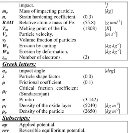
Ain Pipe inlet area. [m2] c Particle concentration [g cm-3] Cp Specific heat capacity [J kg-1 K-1] d Diameter of the pipe. [m] E Applied potential. [V] (SCE) en Normal coeff. of restitution.

F Faraday constant. (96485) [C mol-1] ft Numerical constant. (0.025)

Hs Hardness of the substrate. [Pa] h Thickness of the oxide layer. [m] ho Initial thickness of the oxide. [m] Ip Impact frequency.

[imp cm-2 s-1] ianet Net anodic current density. [A m

-2

] io Exchange current density. [A m-2] Kc Pure corrosion rate. [g m-2 s-1] Kec Total wastage rate. [g m-2 s-1] Ke Pure erosion rate. [g m

-2

s-1] k Material constant. (0.699)

k2 Material constant. (1.398)

-impact. 1] mp Mass of impacting particle. [kg] nc Strain hardening coefficient. (0.3)

RAM Relative atomic mass of Fe. (55.8) [g mol-1] Tm Melting point of the Fe. (1808) [K] Vp Particle velocity. [m s

-1

] vf Volume fraction of particles

WC Erosion by cutting. [kg kg-1] WD Erosion by deformation. [kg kg-1] zm Number of electrons. (2)

Greek letters:

p impact angle [deg] Particle shape factor (0.0)

µ Frictional coefficient (0.1) µf

Critical friction coefficient (Sundararajan)

Pi ratio (3.142)

f Density of the oxide layer. (5240) [kg m-3] p Density of the particle (2650) [kg m-3]

Subscripts:

ap Applied potential.

rev Reversible equilibrium potential.

2. INTRODUCTION

In studies of modelling erosion-corrosion, both finite element (FE) [1] and computational fluid dynamics (CFD) [2-4] techniques have been used to investigate mass loss of materials and to evaluate the effect of various parameters controlling the erosion and corrosion process. However, the majority of these investigations do not introduce a full definition for erosion-corrosion regimes resulting from the interaction between erosion and corrosion. These regimes are very useful in identifying the synergistic, additive, and antagonistic behaviour of this phenomenon in addition to identifying the mechanism of degradation [5].

An approach to identify the transition regimes for the erosion-corrosion process and also to monitor the effects of various parameters was developed by Stack et al. [5] as an extension of earlier work on erosion-corrosion mapping [6-8]. Although 2D mapping is capable of capturing the influence of any particular parameter on erosion-corrosion regime boundaries, it does not give any indication of the combined effect of all the parameters on

these boundaries, nor the metal degradation in a 3D space.

A new methodology was introduced in previous work [9] to study the integrated effect of these parameters together (namely those related to the particle, fluid flow, and environment), on the boundaries of the erosion-corrosion regime and wastage maps by combining the concept of CFD with the erosion-corrosion mapping techniques. Such approach enables us to map the surfaces of any 3D component that are exposed to aqueous slurry flow. Furthermore, it provides a powerful predictive tool for estimating the predominance of various erosion-corrosion regimes.

In this study, a 3D mapping technique is used to investigate the effect of the particle concentration and on the construction of erosion-corrosion mechanism and wastage maps. The effects of particle concentration are evaluated on the regime boundaries. The results are discussed in terms of the applications of this technique to erosion-corrosion in slurry flows in addition to addressing some current limitations.

3. METHODOLOGY

A dilute slurry flow of water-alumina particles of size 10-3[m] and four volume fractions i.e. 0.025, 0.05, 0.075, and 0.1 is ingested through a pipe bend inlet with bore diameter (D) equal to 0.078 [m] and (R D-1) ratio of 1.2.

The CFD simulation generated by FLUENT ver.6.3 [10] uses a finite element based finite volume method to solve the flow governing equations. Table 1 summarizes the equations used, operating and boundary conditions used in this study while Table 2 lists the mechanical and physical properties for the slurry and target material.

[image:2.612.38.295.53.317.2]

Validation of the erosion results is carried out in [9] by comparison to previous experimental work as described elsewhere [11], and is summarised in

[image:3.612.311.559.50.262.2]

for a SS304L stainless steel alloy using Forder’s erosion model [12] as in the case study, and the results were simulated for mild steel using Sundararajan’s second model [13].

Table 1. CFD modeling equations, operating and boundary conditions

Model parameter Water Sand Particles Solver equations Navier-Stokes DPM Turbulence model Standard k-

Wall treatment Standard wall function- no slip

Coupling One way

Operating cond. ambient

[image:3.612.43.282.162.271.2]

Inlet velocity [m s-1] 3.0 3.0

Table 2. Physical and mechanical properties for the slurry and target material

Fluid (water) Particles (alumina) Target (mild steel) density

[kg m-3] 998 2670 7850 particle size

[m] 10

-3

Flow rate

[kg s-1] 14.3 variable

k2 [14] 1.398

Table 3. Comparison between the current study and Experimental and simulation work of Wood et al. [11]

Experimental [11] Simulation [11] current study Erosion rates

[mm3 imp-1]

2.2-5.5 5.5 5.45

3.1. Erosion modelling

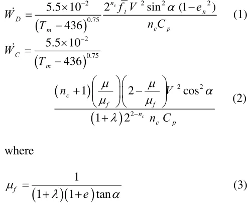
The second model of Sundararajan is divided into two expressions; one accounts for the localised deformation at the impact point, whilst the other addresses the ductile cutting mechanism during the impact. The total erosion rate is the summation of these two mechanisms. The formulation is as follows [13]:

(

)

2 2 2

2

0.75

2 sin (1 )

5.5 10 436 c n t n D c p m

f V e

W n C T α − ₋ × = −

& ₍₁₎

(

)

(

)

(

)

2 0.75 2 2 2 5.5 10 436

1 2 cos

1 2 c

C m c f f n c p W T n V n C

μ μ _α

μ μ λ − − × = − ⎛ ⎞ ⎛ ⎞ + _{⎜ ⎟ ⎜} − _⎟ ⎝ ⎠ ⎝ ⎠ + & (2) where

(

1

)(

11

)

tan f

e μ

λ α

=

+ + (3)

and en is the normal restitution ratio [12] :

2

3 4

0.988 0.78 0.19

0.024 0.027

n

e α α

α α

= − +

− + ₍₄₎

For unit consistency, erosion rates should be converted to [kg m-2 s-1] in line with the calculated corrosion rates below.

3.2. Corrosion rates

3.2.1. Active corrosion model

In the active region, it is assumed that the total corrosion is estimated from knowledge of the dissolution current density from the Butler-Volmer equation: exp (1 ) exp m o anet o m o

z Fr E

R T

i i

z Fr E

R T

β

β

⎡ ⎛ Δ ⎞ ⎤

−

⎢ ⎜ ⎟ ⎥

⎝ ⎠

⎢ ⎥

= ⎢ _{⎛− − Δ ⎞}⎥

⎢ _{⎜ ⎟}⎥

⎢ _{⎝ ⎠}⎥

⎣ ⎦

(5)

where the over-potential E is defined as:

ap rev

E E E

[image:3.612.42.286.332.441.2]

The corrosion rate is therefore given by:

anet

c co

m

RAM i

K K

z F

= = (7)

3.2.2. Repassivation model

For the passivation mechanism, we assume that pure corrosion (Kco) rate is sufficiently low as to

be negligible and the corrosion rate is the additive effect of corrosion enhanced by erosion ( Kc)

[14].

An expression for the corrosion rate in passivation conditions has been introduced [5] and is currently modified to include the effect of the oblique impact [9, 15].

(

)

0.5

₍

₎

2 2

1

1

sin 6

p n

t f p p

s

e

M k h d V

H

ρ

π ρ ⎡⎢ − ⎤⎥ α

=

⎢ ⎥

⎣ ⎦

(8)

The constant k is defined as the mass ratio between the metal and the oxide created during the corrosion reaction, multiplied by the number of moles of metal involved in the reaction and is related to k2 in [14] by definition as (k = k2/2 ).

The thickness of the passive layer h can be assumed to vary with the potential difference and may be given from [16] assuming a linear relationship between the over-potential and passive layer thickness:

(

)

9

3 10

o ap pas

h =h + × − E −E (9)

and: ho=1×10-9 [m].

The unit given by equation (8) is [kg impact-1]. To convert to [kg m-2 s-1], it is multiplied by particle impact flux as outlined in [14]. This can be varied according to the application under investigation. For example, if the flow is homogeneous then particle impact frequency may be used and is given as [17]:

sin

t p

c c

p

M c V

K K

m

α

= Δ = (10)

3.2.3. Erosion-corrosion boundaries

The regime boundaries are determined in terms of the ratio Kc/Ke as

0.1 c

e

K

K < (Erosion dominated) (11)

0.1 c 1 e

K K

≤ < (Erosion-Corrosion dominated) (12)

1 c 10 e

K K

≤ < (Corrosion-Erosion dominated) (13)

10 c

e

K

K ≥ (Corrosion- dominated) (14)

The transition boundaries for the wastage maps are given as follows:

1 ec

K < [mm year-1] (low wastage) (15)

1≤K_ec <10 [mm year-1] (medium wastage) (16)

10 ec

K ≥ [mm year-1] (high wastage) (17)

4. RESULTS

Figure 1 illustrates the Pourbaix diagram for Fe at

T=298 [K] and identifies the possible corrosion

[image:5.612.69.265.53.248.2]

Figure 1: Simplified Pourbaix diagram for Fe at T=298 [K].

To investigate the particle concentration effect, a homogeneous particle distribution in the pipe inlet is assumed and the particle concentration is thus related to the particle mass flow rate according to the relation:

p p p p in

m& =α ρ V A (18)

[image:5.612.313.561.54.398.2]

The simulation was thus run at various particle mass flow rates; namely 0.957, 1.9169, 2.87 and 3.8276 [kg s-1] which are equivalent to particle inlet volume fractions of 0.025, 0.05, 0.075 and 0.0909 respectively.

Figure 2 shows the regime maps at the inner

surfaces of the pipe bend at pH=7 and applied potential E=-0.6 [V] (SCE), illustrating the changes in erosion-corrosion regimes with increasing the particle volume fraction. As the particle volume fraction increases, the erosion rates increases linearly and as a result, the erosion-dissolution and erosion dominated regimes are enlarged. In addition, the dissolution dominated regime reduces with increasing particle volume fraction. This indicates the importance of the volume fraction (or particle concentration) as a factor affecting the erosion-corrosion regimes.

(a)

(b)

(c)

(d)

[image:5.612.314.559.553.728.2]

Figure 2: Regime maps on the outer surface of Fe pipe bend at pH=7 and E= -0.6 [V] (SCE) for particle mass flow rates: (a) 0.957 (b) 1.9169 (c) 2.87 (d) 3.8276 [kg s-1].

Figure 3 illustrates the wastage maps for pH=7

and at applied potential E=-0.6 [V] (SCE) for the same particle mass flow rates listed above as in figure 2. Again the high wastage regime area (red colour region) is increased as the particle mass flow rate increases.

(a)

(c)

[image:6.612.41.288.69.229.2]

(d)

Figure 3: Wastage maps on the outer surface of Fe pipe bend at pH=7 and E= -0.6 [V] (SCE) for particle mass flow rates: (a) 0.957 (b) 1.9169 (c) 2.87 (d) 3.8276 [kg s-1].

5. DISCUSSION

The results indicate that particle volume fraction effects play a significant role in changing the erosion-corrosion regime in 3-D, Figs. 2-3. In the 3-D case, various regimes are observed over the surface, Fig. 2. With increasing volume fraction, the erosion-dominated regime is enhanced. This is due to the increase in erosion rate with increasing particle concentration, shifting the corrosion affected regimes towards those dominated by erosion.

The above trends in the variation of erosion-corrosion regimes on the pipe bend are also observed in earlier work by the current authors [9]. In this work, the significant changes in particle concentration and velocity for the component are identified, resulting in a variation of erosion intensity on the surface. In addition, the local impact angle also changes. Hence, the erosion-corrosion regime variation on the component can be attributed to these factors.

Nonetheless, it should be noted that the variation of the erosion-corrosion regimes only occurs at the pipe bend only and the remaining parts (i.e. entrance and exit straight pipes) exhibit no erosion-corrosion regime change (results not shown). This indicates that the erosion rates at

these regions remain unaffected during the simulation. For the wastage maps, the pipe exit exhibits a minor variation from the medium to the high wastage regime as the particle concentration increases. Hence, the erosion-corrosion mapping technique is a potentially sensitive method of detecting any change in the erosion-corrosion behavior in such environments where changes in component geometry are anticipated.

For the present study, additive erosion-corrosion behaviour is assumed i.e. erosion enhances corrosion and the effect of corrosion on erosion is negligible. The latter effect, the so-called “synergistic/antagonistic” interaction has been attributed to a number of possible mechanisms relating to the material microstructure [18, 19] and it is acknowledged that this is a simplistic assumption. Hence, initial work on mapping the component for the materials above has made such assumptions but future work will address such issues in more detail by assessing materials with composite structures.

Hence, 3D erosion-corrosion maps provide a useful tool for predicting and identification the erosion-corrosion regimes and wastage regions for in-service conditions. The results have indicated significant changes in regimes along the geometry of the component and as a function of increasing particle volume concentration in the pipe. Further work will be to model the effects of other parameters such as oxygen concentration and temperature in addition to extending the range of materials in the model and the synergism/anatagonism between the processes.

6. CONCLUSIONS

• The results indicate changes in erosion-corrosion regimes over the component geometry.

• Increases in particle concentration have a significant effect on the boundaries on the erosion-corrosion regime maps, reducing the corrosion affected regimes in favour of those dominated by erosion.

7. REFERENCES

[1] Griffin, D., Daadbin A., and Datta S., 2004, "The development of a three-dimensional finite element model for solid particle erosion on an alumina scale/MA956 substrate," Wear, 256(9-10), pp. 900-906.

[2] Keating A., and Nesic S., 1999, "Prediction of Two-phase Erosion-corrosion in Bends," Second International Conference on CFD in the Minerals and Process Industries, CSIROMelbourne, Australia, pp. 229-236. [3] Davis C., and Frawley P., 2009, "Modelling of

erosion-corrosion in practical geometries," Corrosion Science, 51(4), pp. 769-775.

[4] Ferng Y., Ma Y., and Chung N., 2000, "Application of local flow models in predicting distributions of erosion-corrosion locations," Corrosion, 56(2), pp. 116-126. [5] Stack M., Corlett N., and Zhou S., 1996,

"Construction of erosion-corrosion maps for erosion in aqueous slurries," Materials Science and Technology, 12(8), pp. 662-672. [6] Stack M., Corlett N., and Zhou S., 1997, "A

methodology for the construction of the erosion-corrosion map in aqueous environments," Wear, 203, pp. 474-488.

[7] Stack M., and Pungwiwat N., 2004, "Erosion-corrosion mapping of Fe in aqueous slurries: some views on a new rationale for defining the erosion-corrosion interaction," Wear, 256(5), pp. 565-576.

[8] Stack M., and Abd El Badia, T., 2006, "On the construction of erosion-corrosion maps for WC/Co-Cr-based coatings in aqueous conditions," Wear, 261(11-12), pp. 1181-1190.

[9] Stack M., Abdelrahman S., and Jana B., 2010, "A new methodology for modelling erosion-corrosion regimes on real surfaces: Gliding down the galvanic series for a range of metal-corrosion systems," Wear, 268(3-4), pp 533-542.

[10] FLUENT Inc., 2006, "FLUENT user's guide, Version 6.3,"Lebanon, NH, USA.

[11] Wood R. J. K., Jones, T., Ganeshalingam J., and Miles N., 2004, "Comparison of predicted and experimental erosion estimates in slurry ducts," Wear, 256(9-10), pp. 937-947.

[12] Forder A., Thew M., and Harrison D., 1998, "A numerical investigation of solid particle erosion experienced within oilfield control valves," Wear, 216(2), pp. 184-193.

[13] Sundararajan G., 1991, "A Comprehensive Model for the Solid Particle Erosion of Ductile Materials," Wear, 149(1-2), pp. 111-127.

[14] Stack M., and Jana, B., 2004, "Modelling particulate erosion-corrosion in aqueous slurries: some views on the construction of erosion-corrosion maps for a range of pure metals," Wear, 256(9-10), pp. 986-1004. [15] Abdelrahman, S., and Stack, M., 2009,

"Some reflictions on a model to predict the erosion rate of the passive film on pure materials," 13th Int. Conf. on Aerospace Science and Aviation Technology, ASAT-2009, Cairo, Egypt.

[16] Graham M., Bardwell J., Sproule G., Mitchell D., and Macdougall, B., 1993, "The Growth and Stability of Passive Films", Corrosion Science, 35(1-4), pp. 13-18.

[17] Lu B., Lue J., 2008, "Correlation between repassivation kinetics and corrosion rate over a passive surface in flowing slurry," Electrochimica Acta, 53(23), pp. 7022-7031. [18] Stack M., Corlett N., and Turgoose S., 2003,

"Some thoughts on modelling the effects of oxygen and particle concentration on the erosion-corrosion of steels in aqueous slurries," Wear, 255, pp. 225-236.