A new meshless interpolation scheme for MLPG_R method

City, University of London Institutional Repository

Citation

:

Ma, Q. (2008). A new meshless interpolation scheme for MLPG_R method.

CMES-Computer Modeling in Engineering & Sciences, 23(2), pp. 75-90.

This is the accepted version of the paper.

This version of the publication may differ from the final published

version.

Permanent repository link:

http://openaccess.city.ac.uk/13213/

Link to published version

:

Copyright and reuse:

City Research Online aims to make research

outputs of City, University of London available to a wider audience.

Copyright and Moral Rights remain with the author(s) and/or copyright

holders. URLs from City Research Online may be freely distributed and

linked to.

City Research Online: http://openaccess.city.ac.uk/ [email protected]

A New Meshless Interpolation Scheme for MLPG_R Method

Q.W. Ma1

Abstract: In the MLPG_R (Meshless Local

Petrove-Galerkin based on Rankine source solution) method, one needs a meshless interpolation scheme for an unknown function to discretise the governing equation. The MLS (moving least square) method has been used for this purpose so far. The MLS method requires inverse of matrix or solution of a linear algebraic system and so is quite time-consuming. In this paper, a new scheme, called simplified finite difference interpolation (SFDI), is devised. This scheme is generally as accurate as the MLS method but does not need matrix inverse and consume less CPU time to evaluate. Although this scheme is purposely developed for the MLPG_R method, it may also be used for other meshless methods.

1

Key words: Simplified finite difference interpolation (SFDI),

MLPG, MLPG_R, nonlinear water waves.

1 Introduction

A meshless method, called Meshless Local Petrove-Galerkin (MLPG) method, has been invented by Atluri and Zhu (1998) and Atluri and Shen (2002) and has been developed into many forms as summarised in Atluri, Liu and Han (2006). This method is based on a local weak form over local sub-domains (circles for two dimensional problems and spheres for three dimensional ones). The success of the MLPG method has been reported in solving fracture mechanics problems [Batra and Ching (2002)], beam and plate bending problems [Atluri and Zhu (2000)], three dimensional elasto-static and -dynamic problems [Han and Atluri (2004a,b)] and some fluid dynamic problems, such as steady flow around a cylinder [Atluri and Zhu (1998)], steady convection and diffusion flow [Lin and Atluri (2000)] in one and two dimensions and lid-driven cavity flow in a two dimensional box [Lin and Atluri (2001)].

In Ma (2005a), the MLPG method was extended to simulating nonlinear water waves and produced some encouraging results. In that paper, the simple Heaviside step function was adopted as the test function to formulate the weak form over local sub-domains, resulting in one in terms of pressure gradient.

In Ma (2005b), the MLPG method was developed into a new form called the MLPG_R method, suitable for modelling nonlinear water waves. In the MLPG_R method, the solution for Rankine sources rather than the Heaviside step function

was taken as the test function. Based on this test function, a weak form of governing equations was derived, which did not contain the gradients of unknown functions, therefore made numerical discretisation of the governing equation relatively easier and more efficient. A semi-analytical technique was also developed to evaluate the domain integral involved in this method, which dramatically reduce the CPU time spent on the numerical evaluation of the integral. Numerical tests showed that the MLPG_R method could be twice as fast as the MLPG method for modelling nonlinear water wave problems.

1 School of Engineering and Mathematical Sciences City University

Northampton Square, London, UK, EC1V 0HB

In the MLPG_R method, the water wave problems are solved using a time-step marching procedure. This starts from a particular instant when the velocity and the geometry of fluid flow are known and then evolves to next time step, at which all physical quantities are updated by solving the governing equations. During each time step, the problem is formulated using a well-known time-split procedure, in which the velocities of particles are updated by

1 *

1

' _’ n

n

p t u u

U

&

& ₍₁₎

where u&n1 is the velocity at time t_n1 , u&* is the intermediate velocity evaluated by the velocity and external

forces in previous time step and is the pressure at time

. The pressure is found by solving

n1

p

1

n

t

*

2 1

u G p pdS

RI I

I

&

³

: w D

SD (2a)

where R_Iis the radius of integration domain :_I, =1 for 2D cases, =2 for 3D cases and Gu&* is defined as

° ° °

¯ °° °

® ­

' '

³ ³³

³ ³

I I

R r R

r

d drd u

t

drd r u t u

G

0 2

0 0 * 0

2

0 *

(*)

cases 3D for sin

2

cases 2D for ,

2

SS S

E T T SD

U

T T S

U

&

(2b)

where ur* is the radial component of the intermediate

velocity u&* .

develop a new meshless interpolation scheme, requiring less computational efforts, and thus to further enhance the overall efficiency of the MLPG_R method.

2 Brief review on meshless interpolation schemes for

MLPG methods

Various available meshless interpolation schemes have been reviewed by Atluri and Shen (2002) and also by Atluri (2005). They include the Shepard function (SF), the partition of unity (PU), the reproducing kernel particle interpolation (RKPM), radial basis function (RBF) and moving least square (MLS) methods. The simplest one among them is the SF method, which is the same as the interpolation of an unknown function used in a moving particle semi-implicit method (MPS) and can suffer a problem of large errors as discussed below. The PU method is more computational expensive and so is not good choice for the family of MLPG methods. The RKPM is equivalent to the MLS method if the basis and weight functions used in them are the same. Atluri and Shen (2002) carried out numerical investigations and demonstrated that the RBFs was not as accurate as the MLS method for the same number of nodes or needed more nodes to achieve the same accuracy. Therefore, the MLS method is more popular than other interpolation schemes for the MLPG methods. It is also the reason why it was utilised by the author in Ma (2005a and 2005b).

For the sake of completeness and convenience of discussions below, the MLS method is outlined here. To be more general, the unknown function is represented by f r& with r&

denoting the position vector of a point, which may also be the

pressure (p) in the MLPG_R method. With the MLS method,

the unknown function f r& can be written as

¦

|

N

J

J J r f

r

f

1 ˆ

&

& _(3a)

where N is the number of nodes that affect the function at

point r&; are nodal variables but not necessarily equal to the nodal values of

J

fˆ

r

f & . In the equation, _J r& is called the interpolation or shape function and is given as

The interpolations given by Eqs. (3a) and (3f) are accurate for a linear function independent on the node distribution. This is a good feature particularly for the problems, such as about nonlinear water waves, involving large deformation of computational domain. Nevertheless, they do have some drawbacks. (1) The interpolation function will not be well

defined if the number of nodes (N) affecting the concerned

point is not large enough. This implies that it may not always work properly when modelling the problems associated with fragment phenomena, such as breaking waves. Although this may be overcome by enlarging the support domain, the larger support domain may lead to over-smoothing and so degrade the accuracy. (2) Interpolation of the function in Eq. (3a) needs the inverse of matrix A, which

is the order of mum. Although m may be only 3 for 2D

case and only 4 for 3D cases, the computational cost spent on it is not negligible due to the fact that the number of points at

>

@

r r

r

r r r r

J T

m

l

lJ l

J

& & &

& & & &

B A

B A

1 1

1

) (

) (

¦

(3b)

with the basis function, assuming to be linear, being

>

, ,

@

[1, , ] )

(r _{1 2 3} x y

T

\ \ \

&

(m=3) for 2D cases

and

>

, , ,

@

[1, , , ] )

(r _{1 2 3 4} x y z

T & _{\ \ \ \}

(m=4) for 3D cases;

and with the matrixes Bx* and Ax* being defined as

>

& & & & & &

@

& &

,

, _{2 2 2}

1 1

1r r r w r r r

w

r

r T

W B

(3c)

and

B W

A r& T r& r& ,

where Wr& and are, respectively, expressed by

»»

» » »

¼ º

« « « « «

¬ ª

J J

J

r r w r

r w

r r

& &

&

& &

&

0

0

0 0

W (3d)

and

>

N

@

T _r& _r& _r&

1, 2 , , , (3e)

which shows each column of the matrix T is the value of

the basis function at a particular point. w

r rJ

& &

in Eq.

(3d) is a weight function. Its specific form will be given later. The gradient of the unknown function is estimated by

¦

’

| ’

N

J

J J r f

r

f

1

ˆ

& &

(3f)

The partial derivatives (or the gradient) of the shape function with respect to y are found by directly differentiating Eq. (3b), that is,

y J T J y T J y T y J

,

1 ,

1 1

,

, AB A B AB (3g)

where A1,y is the partial derivative of A1 (the inverse of

r&

A ), with respect to y (x or z) and is evaluated by

and is J-th column of Matrix B

whose partial derivative is estimated by 1

, 1 ,

1

_{A A A}

A y y BJ

J J J y

J r

y r r

w & & &

B

w w

which the function f r& needs to be estimated is much larger (at least 8 times for 2D and 16 times for 3D) than the total number of nodes when discretising Eq. (2a) and that the computational cost for the inverse of the matrix is

proportional to . (3) The evaluation of the gradient by

direct differentiation as shown in Eqs. (3f) and (3g) is even more expensive due not only to the inverse of matrix but also to the successive multiplication of several matrixes. To avoid the direct differentiation on the interpolation function, Prof. Atluri and his research group suggested a mixed approach in their several recent publications. In particular, Atluri, Liu and Han (2006) describe the following new formulation. The unknown function is still evaluated using Eq. (3a) but its gradient is estimated by a finite difference method. In this method, the components of the gradient are determined by minimising the norm of the unknown function with respect to the gradient components (similar to a least square method) and are expressed (different symbols used in this paper to avoid some confusion with other equations) as

3

m

I IJ

y I

N

J J y I

I

y r H f r r H f r

f &

¦

& 9'& &

1

, (4)

¦

_JN J

y y H

H

1

where f_,yI r&_I is the y-component (y can be changed into x

or z to give other components) of the gradient of f r& at Node I, H=(TW)-1TW , T=[ rI1

&

' , rI2

&

' , rI3

&

' …….

IN

r&

' ], 'r&_IJ r&_J r&_I , W is the same matrix as in Eq. (3d) and is a shrink factor, controlling the position of sample points that are not necessarily the nodes. If the shrink factor

is not equal 1, the value of f

rI rIJ

& & _9'

must be found by Eq. (3a) before estimating the gradient.

Another relevant meshless interpolation is the one used in the moving particle semi-implicit method (MPS) developed by Koshizuka and Oka (1996) and adopted by others [e.g. Koshizuka, Ikeda and Oka, (1999), Heo, Koshizuka and Oka, (2002)]. In the MPS method, a function and its gradient are modelled by

¦

¦

J J J

J J

r r w

r r w r f

r f

0 0

0 & &

& & &

& _(5a)

>

@

₂

0

0 , 0 , 0 0

,

0

r r w r r

r r r f r f r r w

d

f J

J y y J J

J J

J r

y

& & & &

& & & & &

&

&

¦

¦

(5b)

where J represents the neighbour nodes of Point r&₀ ,

r r0

w &_J & is a weight function as mentioned above, is the partial derivative with respect to y (changeable to x or z),

y

f_,

y J

r ,

&

is the component of the position vector in y (x or z)

direction and d is a number of spatial dimensions, equal to 2 in 2D cases and 3 in 3D cases. Although these expressions are very easy to evaluate, they are only rough approximations. This can be seen by the following fact. Eq. (5a) is accurate for any distribution of nodes only if the function is a constant or accurate for a linear function only when the nodes are symmetrical about Point r&₀. The condition of symmetry is not met even if all nodes are located at intersection points of a rectangular grid unless Point r0

&

is also a node, not arbitrary. Eq. (5b) is even worse. In order to give accurate value of the gradient for a linear function, it does not only require that the point (r&₀) must be a node and all nodes lie on intersection points of rectangular grid but also require that the grid must be square. To remove the restriction to the square grid, <RRQ .RVKL]XNDDQG2NDsuggested another expression for the gradient, i.e.

>

@

₂

0

0 , 0 , 0 ,

0 ,

1

0

r r w r r

r r r f r f n

f J

J y y J J

J y

r y

& & & &

& & & &

&

¦

(5c)

where

¦

J

J J

y y J

y wr r

r r

r r

n ₀

2 0

2 , 0 , ,

0

& & & &

& &

.

Similarly, this one is not accurate either for a linear function unless Point r0

&

and all the nodes lie on the intersection points of a rectangular (not necessarily being square) grid. Nevertheless, if the linear function is one dimensional, Eq. (5c) does not depend on the nodes distribution to give accurate results but this feature is rarely useful because problems we consider are generally two or three directional. If Eq. (5b) or (5c) is used to evolve the velocity in Eq. (1) for an irregular distribution of nodes, large errors may be caused. Based on the discussions above, it could be seen that interpolations used in the MPS method are not as good as the corresponding expressions in the MLS formulation in terms of accuracy. The problems with Eq. (5a) and Eq. (5b) or (5c) may become severe if they are used to model the violent water waves, in which it is impossible to keep all the nodes at the intersection points of rectangular grids. If they are really used in such cases, much more number of nodes must be required to achieve the same accuracy, compared with the MLS formulation. However, they are cheaper to compute than those in the MLS scheme mainly because matrix inverse is not involved.

3 Simplified finite difference interpolation (SFDI)

scheme

time to evaluate. This scheme will be particularly useful for the MLPG_R method, in which the values of unknown pressure have to be evaluated at a large number of points when discretising Eq. (2a), as indicated above.

To achieve this, a general functionf r& is expanded into a Taylor series near Point r&₀:

_{0 0}

( ₀2)

0 r r O r r

f r f r

f & & _{’ r}& _˜ && && (6)

Applying the above expression to a set of nodes (J) around

0

r& , multiplying a weight function w

rJ r0

& &

on both sides

and taking the sum of equations at all relevant nodes yields:

_¸¸ ¹ · ¨ ¨ © § ˜ ’

¦

¦

¦

¦

N J J J N J J J r N J J N J J J r r w r r O r r w r r f r r w r f r r w r f 0 2 0 0 0 0 0 0 0 & & & & & & & & & & & & & &

& (7)

where N is the total number of nodes and

0

r

f &

’ is the

gradient of f r& at Point r0

&

. This gives

. 0 0 2 0 0 0 0 0 0 0 0 ¸ ¸ ¸ ¸ ¸ ¹ · ¨ ¨ ¨ ¨ ¨ © § ˜ ’

¦

¦

¦

¦

¦

¦

N J J N J J J N J J N J J J r N J J N J J J r r w r r W r r O r r w r r w r r f r r w r r w r f r f & & & & & & & & & & & & & & & & & &

& (8)

Defining

¦

¦

N J J N J J J r r w r r w r r R 0 0 0 0 & & & & & & & and

_¸¸¸ ¸ ¸ ¹ · ¨ ¨ ¨ ¨ ¨ © §

¦

¦

N J J N J J J r r r w r r w r r O 0 0 2 0

0 _{& &}

& & & & & H ,

one can write the above equation as

0 0 0

0 0

0 N r r

J J N J J J R f r r w r r w r f r

f & & &

& &

& & &

& _{’ ˜ H}

¦

¦

(9)

Omitting the error term

0

r

&

H , the value of the function at

Point r&₀ is approximated by

0

0

0

0 f ₀ R

r r w r r w r f r

f _{N r}

J J N J J J _& & & & & &

& _{’ & ˜}

|

¦

¦

(10)

It is obvious that the error of the approximation is

))

(max( ₀2

0 O rJ r

r

& &

&

H .

In other words, if f r& is a linear function and

0

r

f &

’ is its

accurate gradient, the expression for f r&₀ is accurate. On the other hand, iff r& is a general function, the expression has a second order of accuracy. This is similar to the approximation of the MLS using a linear basis. Nevertheless, the gradient

0

r

f &

’ is generally unknown. Although we may

derive another set of equations for

and solve them

together with Eq. (10) as in Liszka, Duarte and Tworzydlo (1996), it conflicts with our purpose to derive a shape function that does not require matrix inverse or solution of linear algebraic equations. To circumvent the difficulty, it is suggested that

r0 f & ’ 0 r f &

’ is replaced by , where

I

r

f &

’ rI

& _{is one}

of nodes among r&_J(J=1,2, ……), that is,

0

0

0

0 f R

r r w r r w r f r f I r N J J N J J J _& & & & & &

& _{’ & ˜}

|

¦

¦

(11)

The alternation to the gradient in the above equation is a key point of the new scheme. Because of this, it is called as ‘simplified’ finite difference interpolation (SFDI). It is noted that this alternation does not affect the accuracy of the

expression if f r0

&

is a linear function because

0 r f & ’ = I r f &

not affect the order of accuracy for a general function. It is also noted that r&_I may be the nearest node to Point r&₀ but

not necessary. Of course, the gradient

must be

evaluated to obtain the final form of the shape function. There are variety ways to do so. For example, the method described in the next section may be used but it again needs the solution of a linear algebraic system. In this paper we choose to estimate it by using Eq. (5d), i.e., the components

of is approximated by

rI f & ’ I r f & ’

>

@

¦

_z N I J I J I J y I y J I J y I r

y w r r

r r r r r f r f n f I & & & & & & & &

& , ,₂

, , 1 (12) where

¦

_z N I J I J I J y I y J y

I wr r

r r

r r

n _{& &} & &

& & 2 2 , , ,

with y changed into x or z to give other components of the gradient. As already noted for Eq. (5), the gradient expressed by Eq. (12) is not accurate to the order of

)

(max(r r₀2

O &_J & unless all the nodes are uniformly distributed around Point r0

&

and thus may not be used for estimating the velocity directly. However, in Eq. (11), the

term has higher order than the first term and so

the error in the estimation of

may not significantly

degrade the accuracy of 0 R f I r & & _˜ ’

rI f & ’ 0 r

f & . This will be confirmed by the numerical tests in later sections. Substituting Eq. (12) into (11), it follows that

J

N

J

I J r r f r

r

f &

¦

) & & &

1 0

0 ; (13)

where )_J

r&₀;r&_I

is the shape function in the SFDI interpolation and is defined by

¦

¦

z ) N I J I J IJ I J IJ N J J J I

J B r B r

r r w r r w r

r & &

& & & & & & , 0 , 0 0 0

0; 1 G G

Where ¯ ® ­ zJ I J I IJ 0 1 G ,

_¦

d k x I x J x I x I J I J I

J k k

k

k _{r r}

n R r r r r w r B 1 , , , , 0 2 , 0 & & & & & & & & _, and

¦

¦

N J J N J J x x J x r r w r r w r r R k k k 0 0 , 0 , , 0 & & & & & & & ,

where d is still the number of spatial dimensions as defined above and for k=1,2 and 3 is x, y and z, respectively. It may be noted that the methodology to formulate the above interpolation function is some what similar to that for formulating the consistent SPH approximation [Chen and Beraun (2000)]. However there are three differences. (1) Eq. (6) is integrated over a domain in SPH approximation rather than taken as the weighted sum. (2) The integration must be performed on a mesh while Eq. (7) is based only on the weight function. (3) Therefore, the consistent SPH approximation relies on a background mesh. Comparatively, Eq. (13) is a truly meshless expression. (4) The consistent SPH approximation for a function did not have the second term, i.e., similar to the form used in the MPS method.

k

x

4 Gradient interpolation

As pointed out before, the velocity evolvement of particles in Eq. (1) for the MLPG_R method requires the evaluation of pressure gradient. In this section, the interpolation for the gradient is developed by using the similar method to the above in order to replace Eq. (3f) with the new one eliminating the necessity of multiplications of several matrixes . For this purpose, Eq. (6) is rewritten as

r f r0 f ₀ r r0

O(r r02)

f &_J & _{’ r}& _˜ &_J & &_J&

Multiplying

₀

2 0 , 0 , r r w r r r r J J x x

J m m & &

& &

& &

on both sides, taking

the sum of equations at all the relevant nodes and ignoring the error term, it follows that

>

@

¦ ¦

¦

¦

z N J J J x x J d m k k r x k x J N J r x J J x x J N J J J x x J J r r w r r r r f r r f r r w r r r r r r w r r r r r f r f m m k k m m m m m 0 2 0 , 0 , , 1 , , 0 , , 0 2 0 2 , 0 , 0 2 0 , 0 , 0 0 0 & & & & & & & & & & & & & & & & & & & & & & & &

Alternatively, we have

m d m k k r x mk r

x a f C

f

k m 0,

, 1 , , 0 , 0 0

¦

z

&

& (m=1, 2,…, d) (14)

>

@

¦

N

J

J J

x x J J

x

m w r r

r r

r r r f r f n

C m m

m

0 2

0 , 0 , 0 ,

0 , 0

1 & &

& &

& & & &

and

¦

N

J

J J

x x J x x J x

mk w r r

r r

r r r r

n

a m m k k

m

0 2

0 , 0 , , 0 ,

, 0 , 0

1 & &

& &

& & & &

.

Solving the system in Eq. (14), one can find the gradient components. For example, in 2D cases, they are

21 , 0 12 , 0

2 , 0 12 , 0 1 , 0 ,

1

0 a a

C a C fx _r

&

and

21 , 0 12 , 0

2 , 0 21 , 0 2 , 0 ,

1

0 a a

C a C f

r y

& .

In 3D cases, Eq. (14) can be generally written as

> @

A

^ `

F [C]

^ `

Gf

where

^ `

F «¬ª f,x r0 f,y r0 f,z r0º»¼T

,

, & &

& ,

^ `

>

T

J f r

r f r f r f r f r f

f &₁ &₀ , &₂ &₀ ,, & &₀ ,

@

G ,

]

[C is an 3×N matrix with its components defined as

0 2

0 , 0 ,

, 0

1

r r w r r

r r

n

C J

J x x J x

mJ m m

m

& & &

& & &

,

> @

A is an 3×3 matrix with its entries given by

m k

a

A_{mk 0,mk} z

and A_mm 1.

At last, the gradient components may be written as

>

@

¦

*

N

J

J mJ

r

x r f r f r

f

m 1

0 0

,

~

0

& & &

& (15a)

with

& ~ ₁₂₃ ~

1

0 A C J , ,

r

d

k

kJ mk mJ

*

¦

, (15b)

where

> @

A~ is the inverse matrix of

>

A

@

, i.e.

> @

A~

> @

A1 .

0 ~

r

mj

&

* is the shape function for gradient components.

Compared with Eqs. (3f) and (3g) in the MLS method, the expressions in Eq. (15) needs to solve a smaller number of equations, to evaluate the multiplication of a smaller number

of matrixes, and therefore require less CPU time, making the method more efficient particularly in 3D cases.

It is easy to deduce that if f r& is linear Eq. (15) gives exact value of gradient components, independent of the distribution of nodes. This equation may be used in Eq. (11) to formulate the shape function for the interpolation of the unknown function with sacrifice to CPU time and with slight improvement to the accuracy. Another point is worthy to be pointed out is that Eq. (15) become equivalent to Eq. (4) if the shrink factor is taken as 1. Therefore the same expression of the gradient is obtained by using two different methods. In addition, for some special cases, such as all neighbour nodes lying on a special line in 2D cases or in a special plane

in 3D cases,

> @

A1may not exist. This difficulty may be

overcome simply by making (the SFDI is reduced

to Eq, (5c) ) for the node concerned. It should be noted that this difficulty is not only with the SFDI method but also with schemes such as Eq. (4) or the MLS method. The real reason is that for such a special distribution of neighbour nodes, one actually attempts to model the gradient in a low-dimensional space (e.g. 2D) using a function defined in a high-dimensional space (e.g. 3D).

0 ,

0mk

a

5 Convergent rate

In this section, investigations will be made into the convergent rate of the new shape functions in Eqs. (13) and (15) by comparing with their counterparts in other two methods through numerical tests on assumed functions. Although they can be used for any problem, the numerical tests will be carried out on 2D problems.

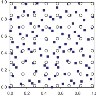
The computational domain for the tests is chosen as a square with the length of sides being 1. The nodes, at which the nodal values f r&_J are defined, are irregularly distributed by using quasi-random number [see for example, Faure, H. (1990)]. A typical node distribution is illustrated in Fig 1.

0.0 0.2 0.4 0.6 0.8 1.0

[image:7.595.342.500.540.699.2]

0.0 0.2 0.4 0.6 0.8 1.0

Fig. 1 Example of distributions of nodes and interpolation points (Hollow circles: interpolation points; Solid squares:

Generally, as noted before, Eq. (13) is used in the MLPG_R method to discretise Eq. (2), giving the relationship between a function value at any point and nodal values of the same function at nodes. On the other hand, Eq. (15) is employed to estimate the pressure gradient of the same function at nodes by using its nodal values for evolving the velocity in Eq. (1). Therefore, different approaches should be adopted when investigating the convergent rate of Eq. (13) and Eq. (15).

To investigate the convergent rate of Eq. (13), the assumed functions are interpolated by the equation at a set of points. These interpolation points are not necessarily coincided with any node and the number of the points is not necessary the same as the number of nodes. In fact, the number of points in the following tests is fixed as 64 except for Section 5.3. For clarity, these points are denoted by r&_0k while nodes are still denoted by r&_Jas above. The distribution of the points is illustrated in Fig. 1. The error of the results of interpolation is defined as

¦

K

k

k k mean f r f r

K

E 1 &₀ &₀ (17)

where Emean is the mean error, f

r0k

&

is the interpolated

value at the interpolation points and f

r&_0k

is the values computed by the formula defining a function at the same point; K is the number of interpolation points.

For investigating the convergent rate of Eq. (15), the gradient of the function is estimated at the nodes by the equation and the error is found by the following expression

¦

M

J

J y J y y

gmean f r f r

M

E _, 1 _, & _, & (18)

where represents the mean error of the y-component

of the gradient,

y gmean

E ,

J y r

f_, & is the approximate value of the y -component of the gradient obtained by interpolation,f_,y r&_J

is its counterpart computed by the formula defining the function and M is the total number of nodes. The mean error

of the x-component of the gradient can be estimated in the

same way by replacing y with x.

There are many options for the weight function. It is not necessary to use the same one for estimating unknown functions and for estimating their gradients. In this paper, however, we mainly concern about the convergent rate of different formulations rather then the best weight function. Therefore, the spline function is employed in all the cases, i.e.,

° ° ° ° °

¯ °° ° ° °

® ­

! '

d ' d

¸ ¸ ¹ · ¨ ¨ © § ' ¸ ¸ ¹ · ¨ ¨ © § ' ¸ ¸ ¹ · ¨ ¨ © § '

'

1 0

1 0

3

8 6

1

4 3

2

I I I I

I

h r

h r h

r

h r

h r

r w

& & & &

&

&

where 'r& is the distance of two points as defined before

and is the size of the support domain of the weight

function which is given by with being the

distance between Node I and the fourth nearest neighbour

and with k being a scale factor.

I

h

I I kh

h ₄ h_4I

5.1 Case 1 – second order polynomial function

The fist considered is a polynomial function of second order

expressed by . Its gradient components are

easy to find and is not written out here. The total number (M) of nodes in the square domain described above is selected as 25, 100, 400, 900 or 1600, respectively, in different runs. The convergent rates for interpolation of the function at 64 points by using three methods are shown in Fig. 2, where the scale factors for the SFDI and MLS are 2.5 and for the MPS two curves are shown corresponding to the scale factors of 2.5 and 5, respectively. The convergent rates are denoted by the decrease of mean errors defined in Eq. (17) with the increase in the total number of nodes. The figure demonstrates that the errors of all three methods are reduced if more nodes are distributed in the same domain. The rates of reduction in errors of the SFDI and MLS methods are similar while the rate of the MPS is considerably slow compared with other two methods. This obviously indicates that the SFDI and MLS can achieve the similar level of accuracy while the MPS is not as robust as other two when nodes are irregularly distributed.

2

2 ₃

2

1 x y

f

ORJ0

ORJ

(PHDQ

[image:8.595.306.495.93.203.2]

6)',N 0/6N 036N 036N

[image:9.595.350.512.110.236.2]

Fig. 3 shows the convenient rates of the three methods for estimating the gradient components or partial derivative of

the polynomial function. The value of ( is similar

and is not necessary to show) is computed by using Eq. (15), (3f) and (5c), respectively, and the error is yielded by Eq. (18). It can be seen that the errors of both the SFDI and MLS methods are almost the same and decrease with increase in the number of nodes while the MPS loses its reasonableness for the scale factor of 2.5 for the irregular distribution of nodes. The results of the MPS corresponding to the scale factor of 5 seem to be more reasonable but still far worse than those of other two methods. This example demonstrates that Eq. (5c) from the MPS is not always reliable to estimate the gradient and should not be considered as an option for problems with a large deformation where original regular distribution of nodes may become irregular.

y

f_, f_,x

ORJ0

O

R

J(PHD

Q\

6)',N 0/6N 036N 036N

Fig. 3 The convergent rate of three methods for estimating the gradients

One may notice from the figures that the scale factor may affect the convergent property of these methods. Investigations are then made by selecting different scale factors. The results of the SFDI for the different scale factors of 1.8, 2.1, 2.5 and 3.0 are shown in Fig 4 and Fig. 5. It is interesting to see that convergent rate of this methods are not very sensitive to the scale factors. This may be considered as another advantage of the SFDI because people may not always know the optimised values of the scale factor.

ORJ0

OR

J(

PHD

Q

[image:9.595.93.253.298.423.2]

6)',N 6)',N 6)',N 6)',N

Fig. 4 Convergent rate of the SFDI for interpolating the polynomial function (Eq. (13))

ORJ0

ORJ(PHDQ\

6)',N 6)',N 6)',N 6)',N

Fig 5 Convergent rate of the SFDI for estimating the gradients (Eq. (15))

The convergent rate of the MLS method corresponding to the scale factors of 1.8, 2.1, 2.5 and 3.0 are depicted in Fig. 6 and Fig. 7. Compared with the results in Figs. 4 and 5, the reduction in the errors for interpolating the polynomial function seems to be faster here with the decrease of the scale factor and the reduction in the errors for estimating the gradients for different scale factors seem to be the same when the total number of nodes is large enough. However, when the scale factor is small and the total number of nodes is not big enough, the results of the MLS is not as good as those of the SFDI. This is clearly illustrated by the cases with the scale factor being 2.1 or less. That is because the number of neighbour nodes at some points is not large enough when the scale factor and so support domain is small. One may deduce from this fact that the MLS scheme may not work well in some sub-areas where nodes are thinly scattered even though total number of nodes in the whole domain may be large enough. Such circumstances may happen to simulating violent flow of fluids, e.g. breaking waves. At the beginning, one may distribute enough number of nodes in the whole domain. However when waves become breaking, nodes in the front area of the breaking waves may become very fragmentary. The investigation in this subsection seems to show that the SFDI may yields better results than the MLS when modelling such waves.

-3.0 -2.5 -2.0 -1.5 -1.0 -0.5 0.0

1.00 2.00 3.00 4.00

log(M )

lo

g

(Emean

)

[image:9.595.346.502.585.704.2]

M LS k=1.8 M LS k=2.1 M LS k=2.5 M LS k=3.0

[image:9.595.91.253.601.720.2]

-2.0 -1.5 -1.0 -0.5 0.0

1.00 2.00 3.00 4.00

log(M )

lo

g

(E

m

ea

n,

y)

[image:10.595.356.511.97.213.2]

M LS k=1.8 M LS k=2.1 M LS k=2.5 M LS k=3.0

Fig 7 Convergent rate of the MLS for estimating the gradients (Eq. (3f))

The results obtained by the MPS method are depicted in Fig. 8 and Fig. 9. As the convergent property of this method seems to be sensitive to the scale factor as illustrated in Figs. 2 and 3, a larger range of the factor, from 1.5 to 12, is investigated. These figures show that the results of the MPS can be very different if the scale factor is not properly selected. They also show that the best scale factor for interpolation of the function is different from that for estimating the gradients. The former is near 1.5 and the latter near 5 for the second-order polynomial. The requirement of a large scale factor by the MPS method means that a large number of neighbour nodes are involved in the evaluation of the gradients. That does not only increase the computational costs but also degrade the accuracy in the region where the gradient varies rapidly. Therefore, a great care must be taken when choosing the scale factor for the MPS method.

ORJ0

OR

J

(P

HD

Q

[image:10.595.95.253.111.230.2]

036N 036N 036N 036N 036N 036N 036N 036N 036N

Fig. 8 Convergent rate of the MPS for interpolating the polynomial function (Eq.(5a))

ORJ0

ORJ(P

HDQ\

036N 036N 036N 036N 036N 036N 036N 036N 036N

Fig. 9 Convergent rate of the MPS for estimating the gradients (Eq. (5c))

5.2 Case 2 – cosine function

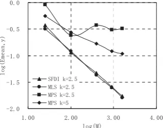
The second function considered is defined byf cos(0.5Sx)cos(0.5Sy). The same investigations as for the polynomial function are made for this cosine function, i.e. the computational domain, the number of nodes and the values of the scale factor are all the same. The convergent rates for interpolating the cosine function and for estimating its derivative by the three methods are plotted in Fig. 10 and Fig. 11, respectively. Compared Fig. 10 with Fig. 2 and Fig. 11 with Fig. 3, it can be seen that the curves in the corresponding figures are largely similar, though specific values are not the same due to different functions concerned with.

-3.5 -3.0 -2.5 -2.0 -1.5 -1.0

1.00 2.00 3.00 4.00

log(M)

log(

E

m

ea

n)

[image:10.595.349.511.450.573.2]

SFDI k=2.5 M LS k=2.5 M PS k=2.5 M PS k=5.0

[image:10.595.91.251.482.606.2]

-2.5 -2.0 -1.5 -1.0 -0.5

1.00 2.00 3.00 4.00

log(M )

lo

g

(E

m

ean

,y

)

[image:11.595.96.253.94.217.2]

SFDI k=2.5 M LS k=2.5 M PS k=2.5 M PS k=5.0

Fig. 11 Convergent rates of three methods for estimating the gradient of cosine function

-3.5 -3.0 -2.5 -2.0 -1.5 -1.0

1.00 2.00 3.00 4.00

log(M)

lo

g

(Em

ea

n

)

[image:11.595.354.512.157.276.2]

SFDI k=1.8 SFDI k=2.1 SFDI k=2.5 SFDI k=3.0

Fig. 12 Convergent rate of the SFDI for interpolating the cosine function (Eq. (13))

-2.5 -2.0 -1.5 -1.0 -0.5

1.00 2.00 3.00 4.00

log(M)

lo

g

(E

m

e

an,

y)

SFDI k=1.8 SFDI k=2.1 SFDI k=2.5 SFDI k=3.0

Fig. 13 Convergent rate of the SFDI for estimating the gradient of cosine function (Eq. (15))

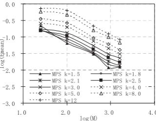
The effects of the scale factors on the convergent rates for the cosine function are also looked at. All the results are presented in Fig. 12 to Fig. 17. These figures seem to support the following conclusions obtained by using the polynomial function. 1) The results of the SFDI are not sensitive to the scale factors. 2) The MLS method generally works well but may not be as good as the SFDI when the scale factor has a small value and when the total number of nodes is not large enough. 3) The results of the MPS method

do not converge as fast as those of other two methods and are sensitive to the scale factors. The best scale factors are different for interpolating the function and for estimating the gradient (1.5 for the former and 8 for the later in this case).

-3.5 -3.0 -2.5 -2.0 -1.5 -1.0

1.00 2.00 3.00 4.00

log(M)

lo

g

(E

m

ean

)

[image:11.595.100.263.283.407.2]

M LS k=1.8 M LS k=2.1 M LS k=2.5 M LS k=3.0

Fig. 14 Convergent rate of the MLS for interpolating the cosine function (Eq. (3a))

-2.5 -2.0 -1.5 -1.0 -0.5

1.00 2.00 3.00 4.00

log(M)

lo

g

(E

m

e

an,

y)

M LS k=1.8 M LS k=2.1 M LS k=2.5 M LS k=3.0

Fig. 15 Convergent rate of MLS for estimating the gradient of cosine function (Eq. (3f))

-3.8 -3.3 -2.8 -2.3 -1.8 -1.3 -0.8

1.00 2.00 3.00 4.00

log(M )

lo

g

(Emean

)

M PS k=1.5 M PS k=1.8

M PS k=2.1 M PS k=2.5

M PS k=3.0 M PS k=4.0

M PS k=5.0 M PS k=8.0

M PS k=12

[image:11.595.350.514.323.442.2] [image:11.595.99.263.477.602.2] [image:11.595.353.511.494.611.2]

-2.5 -2.0 -1.5 -1.0 -0.5

1.00 2.00 3.00 4.00

log(M )

lo

g

(Em

ean

,y

)

M PS k=1.5 M PS k=1.8

M PS k=2.1 M PS k=2.5

M PS k=3.0 M PS k=4.0

M PS k=5.0 M PS k=8.0

[image:12.595.102.262.96.218.2]

M PS k=12

Fig. 17 Convergent rate of the MPS for estimating the gradient of cosine function (Eq.(5c))

5.3 CPU time

As has been seen, the SFDI can be as accurate as the MLS method. Based on the discussions in Sections 3 and 4, one has known that the SFDI should need less CPU time than the MLS method for a same problem. In this section, the ratio of CPU time required by the SFDI to that by the MLS method will be quantified. For this purpose, calculations of interpolating the polynomial function and estimating its gradient are performed 100 times on the same computer (a Laptop with 1 GB RAM and 1.8 GHz processor) by using the two methods with the scale factor of 2.5. To find the ratio of CPU time for interpolating the function, the total number (M) of nodes is selected as 1600 but the number of interpolation

points (K) varies from 64 to 6400. To find the ratio of CPU

time for estimating the gradient at nodes, the total number of nodes varies from 400 to 1600. Fig. 18 shows the ratio of CPU time for interpolating the function used by the SFDI to that by the MLS method while Fig. 19 gives the ratio of CPU time for estimating the gradient used by the SFDI to that by the MLS method. It can be seen that the ratio in Fig. 18 is about 0.76 while the ratio is only 0.16 in Fig. 19. In addition to this, the ratio seems not to vary significantly with the change in the number of interpolation points or nodes. It is noted that the specific values of the ratios may depend on the scale factor. However, according to numerical tests (not given here), it is found that reduction in the scale factor tends to decrease the ratios. It is also noted that both ratios should be smaller for 3D cases based on discussions in Sections 3 and 4.

6 Conclusions

In this paper, a new meshless interpolation scheme, named as the SFDI, for the MLPG_R method is developed and numerically investigated. This method is derived by using the Taylor series with ignoring the terms of second and higher order derivatives and is therefore of second order accuracy. Based on the numerical tests, one observes the following features of the scheme. (1) The SFDI is as accurate as the MLS method generally but may be more accurate than the later when the number of neighbour nodes is small. (2) The SFDI needs considerably less CPU time to

evaluate than the MLS. (3) The scheme is not sensitive to the scale factors. (4) It is much more accurate than the scheme used in the MPS method when nodes are irregularly distributed. Although this scheme is purposely developed for the MLPG_R method, it may also be used for interpolation of a function and calculation of its gradients in the other meshless methods.

0.50 0.63 0.75 0.88 1.00

1 2 3 4

Log(K)

CP

U

Ra

ti

o

Fig. 18 Ratio of CPU time used by the SFDI to that by the MLS for interpolating the function

0.00 0.06 0.12 0.18 0.24

2.5 2.75 3 3.25 3.5

Log(M )

CP

U

R

at

[image:12.595.352.497.193.320.2]

io

Fig. 19 Ratio of CPU time used by the SFDI to that by the MLS method for estimating the gradient

Acknowledgement

This work is sponsored by The Leverhulme Trust, UK, to which the author is most grateful.

References

Atluri ,S.N.; Shen ,S. (2002): The Meshless Local Petrove-Galerkin (MLPG) Method: A Simple & Less-costly Alternative to the Finite Element and Boundary Element

Methods, CMES: Computer Modeling in Engineering &

Sciences, Vol. 3 (1), pp. 11-52.

Atluri, S.N.; Zhu, T. (1998): A New Meshless Local Petrov-Galerkin (MLPG) Approach in Computational Mechanics,

Computational Mechanics, Vol. 22, pp. 117-127.

[image:12.595.354.502.377.507.2]

Atluri, S.N.; Liu, H.T.; Han, Z. D. (2006): Meshless Local Petrov-Galerkin (MLPG) Mixed Finite Difference Method

for Solid Mechanics, CMES: Computer Modeling in

Engineering & Sciences, Vol. 15, No.1, pp. 1-16.

Koshizuka, S.; Oka, Y. (1996): Moving-Particle Semi-Implicit Method for Fragmentation of Incompressible Fluid, Nuclear Science and Engineering, 123, pp. 421-434. Koshizuka, S., Ikeda, Y., Oka, Y., (1999): Numerical

analysis of fragmentation mechanisms in vapour

explosions, Nuclear Engineering and Design, 189, pp.

423–433. Chen, J. K.; Beraun, J. E. (2000): A generalized smoothed

particle hydrodynamics method for nonlinear dynamic

problems, Computer Methods in Applied Mechanics and

Engineering, Vol. 190, Issues 1-2, pp. 225-239. Liszka, T. J.; Duarte, C. A. M.; Tworzydlo, W. W.(1996):

hp-Meshless cloud method, Computer Methods in Applied

Mechanics and Engineering, Vol. 139, 263-288. Faure, H. (1990): Using permutations to reduce discrepancy.

J. Comp. Appl. Math., 31:97-103, 1990.

Ma, Q.W., (2005a): Meshless Local Petrov-Galerkin Method for Two-dimensional Nonlinear Water Wave Problems.

Journal of Computational Physics, Vol. 205, Issue 2, pp. 611-625.

Han, Z. D.; Atluri, S. N. (2004a): Meshless Local Petrov-Galerkin (MLPG) Approach for 3-Dimensional

Elasto-dynamics, Computers, Materials & Continua, Vol. 1 (2),

pp. 129-140.

Han, Z. D.; Atluri, S. N. (2004b): Meshless Local Petrov-Galerkin (MLPG) Approaches for Solving 3D Problems in

Elasto-statics, CMES: Computer Modeling in Engineering

& Sciences, Vol. 6 (2), pp. 169-188.

Ma, Q.W., (2005b): MLPG Method Based on Rankine Source Solution for Simulating Nonlinear Water Waves,

CMES: Computer Modeling in Engineering & Sciences, Vol. 9, No. 2, pp. 193-210.

Heo, S., Koshizuka, S. and Oka, Y., (2002): Numerical analysis of boiling on high heat-flux and high sub-cooling

condition using MPS-MAFL, International Journal of

Heat and Mass Transfer, 45, pp. 2633–2642.

Yoon, H.Y., Koshizuka, S., Oka, Y., (2001): Direct calculation of bubble growth, departure, and rise in

nucleate pool boiling, International Journal of Multiphase