The simple harmonic urn

Crane, E. and Georgiou, N. and Volkov, Stanislav and Wade, Andrew and

Waters, R.J. (2011) The simple harmonic urn. Annals of Probability, 39

(6). 2119–2177. , http://dx.doi.org/10.1214/10-AOP605

This version is available at https://strathprints.strath.ac.uk/29125/

Strathprints is designed to allow users to access the research output of the University of Strathclyde. Unless otherwise explicitly stated on the manuscript, Copyright © and Moral Rights for the papers on this site are retained by the individual authors and/or other copyright owners. Please check the manuscript for details of any other licences that may have been applied. You may not engage in further distribution of the material for any profitmaking activities or any commercial gain. You may freely distribute both the url (https://strathprints.strath.ac.uk/) and the content of this paper for research or private study, educational, or not-for-profit purposes without prior permission or charge.

Any correspondence concerning this service should be sent to the Strathprints administrator:

[email protected]

The Strathprints institutional repository (https://strathprints.strath.ac.uk) is a digital archive of University of Strathclyde research outputs. It has been developed to disseminate open access research outputs, expose data about those outputs, and enable the

The simple harmonic urn

Edward Crane∗ Nicholas Georgiou∗ Stanislav Volkov†,‡ Andrew R. Wade§ Robert J. Waters∗

9 August 2010

Abstract

We study a generalized P´olya urn model with two types of ball. If the drawn ball is red it is replaced together with a black ball, but if the drawn ball is black it is replaced and a red ball is thrown out of the urn. When only black balls remain, the rˆoles of the colours are swapped and the process restarts. We prove that the resulting Markov chain is transient but that if we throw out a ball every time the colours swap, the process is recurrent. We show that the embedded process obtained by observing the number of balls in the urn at the swapping times has a scaling limit that is essentially the square of a Bessel diffusion. We consider an oriented percolation model naturally associated with the urn process, and obtain detailed information about its structure, showing that the open subgraph is an infinite tree with a single end. We also study a natural continuous-time embedding of the urn process that demonstrates the relation to the simple harmonic oscillator; in this setting our transience result addresses an open problem in the recurrence theory of two-dimensional linear birth and death processes due to Kesten and Hutton. We obtain results on the area swept out by the process. We make use of connections between the urn process and birth-death processes, a uniform renewal process, the Eulerian numbers, and Lamperti’s problem on processes with asymptotically small drifts; we prove some new results on some of these classical objects that may be of independent interest. For instance, we give sharp new asymptotics for the first two moments of the counting function of the uniform renewal process. Finally we discuss some related models of independent interest, including a ‘Poisson earthquakes’ Markov chain on the homeomorphisms of the plane.

Keywords: Urn model, recurrence classification, oriented percolation, uniform renewal process, two-dimensional linear birth and death process, Bessel process, coupling, Eulerian numbers.

AMS subject classification: Primary: 60J10; Secondary: 60J25, 60K05, 60K35.

1

Introduction

Urn models have a venerable history in probability theory, with classical contributions having been made by the Bernoullis and Laplace, among others. The modern view of many urn models is as prototypical reinforced stochastic processes. Classical urn schemes were often employed as ‘thought experiments’ in which to frame statistical questions; as stochastic processes, urn models have wide-ranging applications in economics, the physical sciences, and statistics. There is a large literature on urn models and their applications — see for example the monographs [20, 30]

∗_{Heilbronn Institute for Mathematical Research, Department of Mathematics, University of Bristol, Bristol}

BS8 1TW, UK †

Department of Mathematics, University of Bristol, Bristol BS8 1TW, UK ‡

Corresponding author

and the surveys [25, 34] — and some important contributions have been made in the last few years: see e.g. [18, 13].

A generalized P´olya urn with 2 types of ball, or 2 colours, is a discrete-time Markov chain (Xn, Yn)n∈Z₊ onZ₊2, whereZ+:={0,1,2, . . .}. The possible transitions of the chain are specified

by a 2×2 reinforcement matrix A = (aij)2i,j=1 and the transition probabilities depend on the

current state:

P_{((Xn+1, Yn+1) = (Xn+a11, Yn+a12)) =} Xn

Xn+Yn

,

P_{((Xn+1, Yn+1) = (Xn+a21, Yn+a22)) =} Yn

Xn+Yn

. (1)

This process can be viewed as an urn which at timencontainsXnred balls andYnblack balls.

At each stage, a ball is drawn from the urn at random, and then returned together withai1 red

balls andai2 black balls, wherei= 1 if the chosen ball is red andi= 2 if it is black.

A fundamental problem is to study the long-term behaviour of (Xn, Yn), defined by (1), or

some function thereof, such as the fraction of red balls Xn/(Xn+Yn). In many cases, coarse

asymptotics for such quantities are governed by the eigenvalues of the reinforcement matrix A (see e.g. [4] or [5, _§V.9]). However there are some interesting special cases (see e.g. [35]), and analysis of finer behaviour is in several cases still an open problem.

A large body of asymptotic theory is known under various conditions onAand its eigenval-ues. Often it is assumed that all aij ≥0; e.g., A=

1 0

0 1

specifies thestandard P´olya urn,

while A=

a b b a

witha, b >0 specifies aFriedman urn.

In general, the entries aij may be negative, meaning that balls can be thrown away as well

as added, but nevertheless in the literaturetenability is usually imposed. This is the condition that regardless of the stochastic path taken by the process, it is never required to remove a ball of a colour not currently present in the urn. For example theEhrenfest urn, which models the diffusion of a gas between two chambers of a box, is tenable despite its reinforcement matrix

−1 1

1 −1

having some negative entries.

Departing from tenability, the OK Corral model is the 2-colour urn with reinforcement matrix

0 ₋1

−1 0

. This model for destructive competition was studied by Williams and McIl-roy [43] and Kingman [23] (and earlier as a stochastic version of Lanchester’s combat model; see e.g. [42] and references therein). Kingman and Volkov [24] showed that the OK Corral model can be viewed as a time-reversed Friedman urn witha= 0 and b= 1.

In this paper, we will study the 2-colour urn model with reinforcement matrix

A=

0 1 −1 0

. (2)

To reiterate the urn model, at each time period we draw a ball at random from the urn; if it is red, we replace it and add an additional black ball, if it is black we replace it and throw out a red ball. The eigenvalues of A are ±i, corresponding to the ordinary differential equation

˙

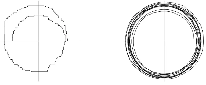
Figure 1: Two sample trajectories of the simple harmonic urn process, starting at (50,0) and running for about 600 steps (left) and starting at (1000,0) and running for 100,000 steps (right).

2

Exact formulation of the model and main results

2.1 The simple harmonic urn process

The definition of the process given by the transition probabilities (1) and the matrix (2) only makes sense forXn, Yn≥0; however, it is easy to see that almost surely (a.s.) Xn<0 eventually.

Therefore, we reformulate the process (Xn, Yn) rigorously as follows.

For z0 ∈ N := {1,2, . . .} take (X0, Y0) = (z0,0); we start on the positive x-axis for

conve-nience but the choice of initial state does not affect any of our asymptotic results. Forn_∈Z_+,

given (Xn, Yn) = (x, y)∈Z2\ {(0,0)}, we define the transition law of the process by

(Xn+1, Yn+1) =

   

  

(x, y+ sgn(x)), with probability _|x||₊x|_|y|,

(x₋sgn(y), y), with probability _|x||₊y|_|y|,

(3)

where sgn(x) = −1,0,1 if x < 0, x = 0, x > 0 respectively. The process (Xn, Yn)n∈Z₊ is an irreducible Markov chain with state-space Z2_{\ {(0,0)}.}

Let ν0:= 0, and recursively define stopping times

νk := min{n > νk−1 : XnYn= 0}, (k∈N),

where throughout the paper we adopt the usual convention min∅ := ∞. Thus (νk)k∈N is the sequence of times at which the process visits one of the axes.

It is easy to see that everyνk is almost surely finite. Moreover, by construction, the process

(Xνk, Yνk)k∈N visits in cyclic (anticlockwise) order the half-lines {y > 0}, {x < 0}, {y < 0}, {x > 0_}. It is natural (and fruitful) to consider the embedded process (Zk)k∈Z₊ obtained by takingZ0:=z0 and Zk:=|Xνk|+|Yνk|(k∈N).

If (Xn, Yn) is viewed as a random walk onZ2, the process Zkis the embedded process of the

distances from 0 at the instances of hitting the axes. To interpret the process (Xn, Yn) as the

urn model described in Section 1 we need a slight modification to the description there. Starting withz0 red balls, we run the process as described in Section 1, so the process traverses the first

balls, but we switch to using ₋x to count the number of red balls. Now the process traverses the second quadrant via a left/down path until the black balls run out, and so on. In the urn model, Zk is the number of balls remaining in the urn when the urn becomes monochromatic

for thek-th time (k_∈N_).

The strong Markov property and the transition law of (Xn, Yn) imply that Zk is an

irre-ducible Markov chain on N_{. Since our two Markov chains just described are irreducible, there}

is the usual recurrence/transience dichotomy, in that either the process is recurrent, meaning that with probability 1 it returns infinitely often to any finite subset of the state space, or it is transient, meaning that with probability 1 it eventually escapes to infinity. Our main question is whether the processZk is recurrent or transient. It is easy to see that, by the nature of the

embedding, this also determines whether the urn model (Xn, Yn) is recurrent or transient.

Theorem 2.1. The process Zk is transient; hence so is the process (Xn, Yn).

Exploiting a connection between the increments of the process Zk and a renewal process

whose inter-arrival times are uniform on (0,1) will enable us to prove the following basic result. Theorem 2.2. Let n∈N_{. Then}

E_{[Zk+1 |Zk=n] = n+} 2

3+O(e

α1n_{) , (4)}

as n→ ∞, where α1+β1i=−(2.088843. . .) + (7.461489. . .)iis a root of λ−1 + e−λ= 0.

The error term in (4) is sharp, and we obtain it from new (sharp) asymptotics for the uniform renewal process: see Lemma 4.5 and Corollary 6.5, which improve on known results. To prove Theorem 2.1 we need more than Theorem 2.2: we need to know about the second moments of the increments ofZk, amongst other things; see Section 6. In fact we prove Theorem 2.1 using

martingale arguments applied toh(Zk) for a well-chosen functionh; the analysis of the function

h(Zk) rests on a recurrence relation satisfied by the transition probabilities of Zk, which are

related to the Eulerian numbers (see Section 3).

2.2 The leaky simple harmonic urn

In fact the transience demonstrated in Theorem 2.1 is rather delicate, as one can see by sim-ulating the process. To illustrate this, we consider a slight modification of the process, which we call the leaky simple harmonic urn. Suppose that each time the rˆoles of the colours are reversed, the addition of the next ball of the new colour causes one ball of the other colour to leak out of the urn; subsequently the usual simple harmonic urn transition law applies. If the total number of balls in the urn ever falls to one, then this modified rule causes the urn to become monochromatic at the next step, and again it contains only one ball. Thus there will only be one ball in total at all subsequent times, although it will alternate in colour. We will see that the system almost surely does reach this steady state, and we obtain almost sharp tail bounds on the time that it takes to do so. The leaky simple harmonic urn arises naturally in the context of a percolation model associated to the simple harmonic urn process, defined in Section 2.4 below.

As we did for the simple harmonic urn, we will represent the leaky urn by a Markov chain (X_n′, Y_n′). For this version of the model, it turns out to be more convenient to start just above the axis; we take (X′

0, Y0′) = (z0,1), where z0 ∈ N. The distribution of (Xn′+1, Yn′+1) depends

only on (X_n′, Y_n′) = (x, y).

If xy ₆= 0, the transition law is the same as that of the simple harmonic urn process. The difference is whenx= 0 or y= 0; then the transition law is

(X_n′₊₁, Y_n′₊₁) = (x₋sgn(x),sgn(x)) (y= 0).

Now (X_n′, Y_n′) is a reducible Markov chain whose state-space has two communicating classes, the closed class _C =_{(x, y) _∈ Z2 _{:|x|+|y|= 1} and the class {(x, y) ∈} Z2 _{:|x|+|y| ≥ 2}; if}

the process enters the closed class _C it remains there for ever, cycling round the origin. Let τ be the hitting time of the set C, that is

τ := inf_{n_∈Z_:|Xn′_|+|Yn′_{|= 1}.}

Theorem 2.3. For the leaky urn, P_{(τ <∞) = 1. Moreover, for anyε > 0,} E_[τ1−ε_{]< ∞ but} E_[τ1+ε_{] =∞.}

In contrast, Theorem 2.1 implies that the analogue of τ for the ordinary urn process has

P_{(τ =∞)>0 ifz0 ≥2.}

2.3 The noisy simple harmonic urn

In view of Theorems 2.1 and 2.3, it is natural to ask about the properties of the hitting timeτ if at the time when the balls of one colour run out we only discard a ball of the other colour with some probabilityp∈(0,1). For whichp isτ a.s. finite? (Answer: for p≥1/3; see Corollary 2.7 below.)

We consider the following natural generalization of the model specified by (3) in order to probe more precisely the recurrence/transience transition. We call this generalization thenoisy

simple harmonic urn process. In a sense that we will describe, this model includes the leaky urn and also the intermittent leaky urn mentioned at the start of this section. The basic idea is to throw out (or add) a random number of balls at each time we are at an axis, generalizing the idea of the leaky urn. It is more convenient here to work with irreducible Markov chains, so we introduce a ‘barrier’ for our process. We now describe the model precisely.

Let κ, κ1, κ2, . . . be a sequence of i.i.d.Z-valued random variables such that

E_[eλ|κ|_{]<∞, (5)}

for some λ > 0, so in particular E_{[κ] is finite. We now define the Markov chain ( ˜Xn,Y}˜_n)n∈Z

+

for the noisy urn process. As for the leaky urn, we start one step above the axis: let z0 ∈ N,

and take ( ˜X0,Y˜0) = (z0,1). For n∈Z+, given ( ˜Xn,Y˜n) = (x, y)∈Z2\ {(0,0)}, we define the

transition law as follows. If xy₆= 0 then

( ˜Xn+1,Y˜n+1) =

   

  

(x, y+ sgn(x)), with probability _|x||₊x|_|y|,

(x₋sgn(y), y), with probability _|x||₊y|_|y|,

while if x= 0 or y= 0 we have

( ˜Xn+1,Y˜n+1) = (−sgn(y),sgn(y) max(1,|y| −κn)) (x= 0),

( ˜Xn+1,Y˜n+1) = (sgn(x) max(1,|x| −κn),sgn(x)) (y= 0).

In other words, the transition law is the same as (3) except when the process is on an axis at time n, in which case instead of just moving one step away in the anticlockwise perpendicular direction it also moves an additional distanceκnparallel to the axis towards the origin (stopping

distance 1 away if it would otherwise reach the next axis or overshoot). Then ( ˜Xn,Y˜n)n∈Z₊ is an irreducible Markov chain on Z2_{\ {(0,0)}. The case where}P_{(κ = 0) = 1 corresponds to the}

A fundamental random variable is the first passage time to within distance 1 of the origin:

τ := min_{n_∈Z_+:|X˜_n|+|Y˜_{n|= 1}= min{n∈}Z_{+: ( ˜Xn,Y}˜_{n)∈ C}.}

Define a sequence of stopping times ˜νk by setting ˜ν0:=−1 and fork∈N,

˜

νk:= min{n >ν˜k−1: ˜XnY˜n= 0}.

As an analogue of Zk, set ˜Z0 :=z0 and for k∈Ndefine

˜

Zk := max{|X˜1+˜νk|,|Y˜1+˜νk|}=|X˜1+˜νk|+|Y˜1+˜νk| −1;

then ( ˜Zk)k∈Z₊ is an irreducible Markov chain onN. Define the return-time to the state 1 by

τq:= min{k∈N: ˜Zk= 1}, (6)

where the subscriptq signifies the fact that a time unit is one traversal of a quadrant here. By our embedding,τ = ˜ντq.

Note that in the case P_{(κ = 0) = 1, ( ˜Zk)k∈Z}

+ has the same distribution as the original

(Zk)k∈Z₊. The noisy urn withP(κ= 1) = 1 coincides with the leaky urn described in Section 2.2 up until the timeτ (at which point the leaky urn becomes trapped in_C). Similarly the embedded process ˜Zk with P(κ = 1) = 1 coincides with the process of distances from the origin of the

leaky urn at the times that it visits the axes, up until time τq (at which point the leaky urn

remains at distance 1 forever). Thus in the P_{(κ= 1) = 1 cases of all the results that follow in}

this section,τ andτq can be taken to be defined in terms of the leaky urn (Xn′, Yn′).

The next result thus includes Theorem 2.1 and the first part of Theorem 2.3 as special cases.

Theorem 2.4. Suppose thatκ satisfies (5). Then the process Z˜k is

(i) transient if E_[κ]<1/3;

(ii) null-recurrent if 1/3_≤E_[κ]≤2/3;

(iii) positive-recurrent if E_[κ]>2/3.

Of course, part (i) means that P_{(τq <∞)<1, part (ii) that}P_{(τq <∞) = 1 but} E_{[τq] =∞,}

and part (iii) that E_{[τq]<∞. We can in fact obtain more information about the tails ofτq:}

Theorem 2.5. Suppose thatκ satisfies (5) and E_{[κ]≥1/3. Then} E_[τqp_{]<∞ forp <3}E_[κ]−1 and E_[τqp_{] =∞ for p >3}E_[κ]−1.

It should be possible, with some extra work, to show that E_[τqp_{] =∞ when p = 3}E_[κ]−1,

using the sharper results of [2] in place of those from [3] that we use below in the proof of Theorem 2.5.

In the recurrent case, it is of interest to obtain more detailed results on the tail of τ (note that there is a change of time between τ and τq). We obtain the following upper and lower

bounds, which are close to sharp.

Theorem 2.6. Suppose that κ satisfies (5) and E_{[κ]≥ 1/3. Then} E_[τp_{]<∞ for p <} 3E[κ]−1 2 and E_[τp_{] =∞ for p >} 3E[κ]−1

2 .

Corollary 2.7. Suppose that κ satisfies (5). The noisy simple harmonic urn process ( ˜Xn,Y˜n) is recurrent if E_{[κ]≥1/3 and transient if} E_{[κ]<1/3. Moreover, the process is null-recurrent if}

1/3_≤E_{[κ]<1 and positive-recurrent if}E_[κ]>1.

This result is close to sharp but leaves open the question of whether the process is null- or positive-recurrent when E_{[κ] = 1 (we suspect the former).}

We also study the distributional limiting behaviour of ˜Zk in the appropriate scaling regime

when E_{[κ]<2/3. Again the case} P_{(κ= 0) = 1 reduces to the original Zk.}

Theorem 2.8. Suppose that κ satisfies (5) and that E_{[κ]<2/3. Let (Dt)t∈[0,1] be a diffusion} process taking values in R_{+ := [0,∞) with D0 = 0 and infinitesimal mean µ(x) and variance}

σ2_{(x) given for x∈R} + by

µ(x) = 2

3−E[κ], σ

2_{(x) =} 2

3x.

Then as k→ ∞,

(k−1Z˜kt)t∈[0,1]→(Dt)t∈[0,1],

where the convergence is in the sense of finite-dimensional distributions. Up to multiplication by a scalar, Dt is the square of a Bessel process with parameter 4−6E[κ]>0.

Since a Bessel process with parameterγ ∈N_{has the same law as the norm of aγ-dimensional}

Brownian motion, Theorem 2.8 says, for example, that if E_{[κ] = 0 (e.g., for the original urn}

process) the scaling limit of ˜Ztis a scalar multiple of the norm-square of 4-dimensional Brownian

motion, while ifE_{[κ] = 1/2 the scaling limit is a scalar multiple of the square of one-dimensional}

Brownian motion.

To finish this section, consider thearea swept out by the path of the noisy simple harmonic urn on its first excursion (i.e., up to time τ). Additional motivation for studying this random quantity is provided by the percolation model of Section 2.4. Formally, forn_∈N_{let Tn be the}

area of the triangle with vertices (0,0), ( ˜Xn−1,Y˜n−1), and ( ˜Xn,Y˜n), and define A:=Pτn=1Tn.

Theorem 2.9. Suppose thatκ satisfies (5).

(i) Suppose that E_{[κ]<1/3. Then} P_(A=∞)>0.

(ii) Suppose that E_{[κ]≥1/3. Then} E_[Ap_{]<∞ for p <} 3E[κ]−1

3 .

In particular, part (ii) gives us information about the leaky urn model, which corresponds to the case where P_{(κ = 1) = 1, at least up until the hitting time of the closed cycle; we can}

still make sense of the area swept out by the leaky urn up to this hitting time. We then have

E_[Ap_{]< ∞ for p < 2/3, a result of significance for the percolation model of the next section.}

We suspect that the bounds in Theorem 2.9(ii) are tight. We do not prove this but have the following result in the case P_{(κ= 1) = 1.}

Theorem 2.10. Suppose P_{(κ= 1) = 1(or equivalently take the leaky urn). Then} E_{[A] =∞.}

2.4 A percolation model

The simple harmonic urn can be viewed as a spatially inhomogeneous random walk on a directed graph whose vertices are Z2 _{\ {(0,0)}; we make this statement more precise shortly.}

In this section we will view the simple harmonic urn process not as a random path through a predetermined directed graph but as a deterministic path through a random directed graph. To do this it is helpful to consider a slightly larger state-space which keeps track of the number of times that the urn’s path has wound around the origin. We construct this state-space as the vertex set of a graph Gthat is embedded in the Riemann surface _Rof the complex logarithm, which is the universal cover ofR2_{\{(0,0)}. To constructG, we take the usual square-grid lattice}

and delete the vertex at the origin to obtain a graph on the vertex setZ2_{\ {(0,0)}. Make this}

into a directed graph by orienting each edge in the direction of increasing argument; the paths of the simple harmonic urn only ever traverse edges in this direction. Leave undirected those edges along any of the co-ordinate axes; the paths of the simple harmonic urn never traverse these edges. Finally, we let Gbe the lift of this graph to the covering surface _R.

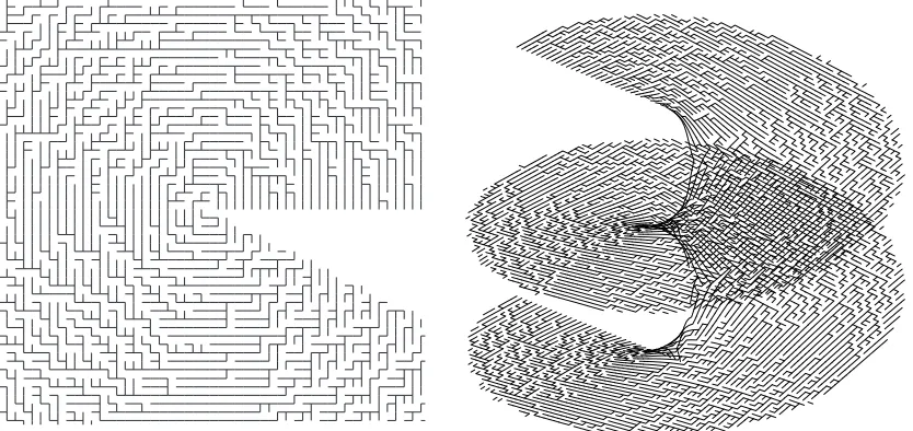
Figure 2: Simulated realizations of the simple harmonic urn percolation model: on a single sheet of _R(left) and on a larger section (right).

We will interpret a path of the simple harmonic urn as the unique oriented path from some starting vertex through a random subgraph H of G. For each vertex v of G the graphH has precisely one of the out-edges from v that are in G. If the projection of v toZ2 _{is (x, y), then}

the graphH contains the edge fromv that projects onto the edge from (x, y) to (x₋sgn(y), y) with probability|y|/(|x|+|y|), and otherwise it contains the edge fromvthat projects onto the edge from (x, y) to (x, y+ sgn(x)). These choices are to be made independently for all vertices v of G. In particular H does not have any edges that project onto either of the co-ordinate axes. The random directed graph H is an oriented percolation model that encodes a coupling of many different paths of the simple harmonic urn. To make this precise, letv0 be any vertex

of G. Then there is a unique oriented path v0, v1, v2, . . . through H. That is, (vi, vi+1) is an

edge ofH for eachi≥0. Let the projection ofvi fromRtoR2 be the point (Xi, Yi). Then the

sequence (Xi, Yi)∞i=0is a sample of the simple harmonic urn process. Ifw0is another vertex ofG,

with unique oriented pathw0, w1, w2, . . ., then its projection toZ2 is also a sample path of the

simple harmonic urn process, but we will show (see Theorem 2.11 below) that with probability one the two paths eventually couple, which is to say that there exist random finite m_≥0 and n_≥0 such that for all i_≥0 we have vi+m =wi+n. Thus the percolation model encodes many

copies of the leaky urn of Section 2.2.

We construct another random graph H′ that is the dual percolation model to H. We begin with the planar dual of the square-grid lattice, which is another square-grid lattice with vertices at the points (m+ 1/2, n+ 1/2),m, n_∈Z_{. We orient all the edges in the direction of decreasing}

argument, and lift to the covering surface R to obtain the dual graph G′. Now let H′ be the directed subgraph of G′ that consists of all those edges of G′ that do not cross an edge of H. It turns out that H′ _{can be viewed as an oriented percolation model that encodes a coupling of} many different paths of the leaky simple harmonic urn.

To explain this, we define a mapping Φ from the vertices of G′ to Z2_{. Let (x, y) be the}

co-ordinates of the projection ofv_∈G′ _{to the shifted square lattice Z}2_{+ (1/2,1/2). Then}

Φ(v) =

x+1

2sgny,−(y− 1 2sgnx)

.

Thus we project from_RtoR2_{, move to the nearest lattice point in the clockwise direction, and}

then reflect in thex-axis. Ifv0 is any vertex ofH′, there is a unique oriented pathv0, v1, v2, . . .

throughH′, this time winding clockwise. Takev0 = (z0−1/2,1/2). A little thought shows that

the sequence (X_i′, Y_i′) = Φ (vi) has the distribution of the leaky simple harmonic urn process.

This is because the choice of edge inH′_{fromvis determined by the choice of edge inH from the} nearest point ofG in the clockwise direction. The map Φ is not quite a graph homomorphism onto the square lattice because of its behaviour at the axes; e.g., it sends (31₂,1₂) and (31₂,₋1₂) to (4,0) and (3,1) respectively. The decrease of 1 in thex-co-ordinate corresponds to the leaked ball in the leaky urn model. If somevi has projection (xi, yi) with|xi|+|yi|= 1, then the same

is true of all subsequent vertices in the path. This corresponds to the closed class_C.

From results on our urn processes, we will deduce the following quite subtle properties of the percolation modelH. Let I(v) denote the number of vertices in the in-graph of the vertex v inH, which is the subgraph ofH induced by all vertices from which it is possible to reachv by following an oriented path.

Theorem 2.11. Almost surely, the random oriented graph H is, ignoring orientations, an infinite tree with a single semi-infinite end in the out direction. In particular, for anyv, I(v)< ∞ a.s. and moreover E_[I(v)p_{]<∞ for anyp <2/3; however,}E_{[I(v)] =∞.}

The dual graph H′ is also an infinite tree a.s., with a single semi-infinite end in the out direction. It has a doubly-infinite oriented path and the in-graph of any vertex not on this path is finite a.s.

2.5 A continuous-time fast embedding of the simple harmonic urn

There is a natural continuous-time embedding of the simple harmonic urn process. Let (A(t), B(t))t∈R₊ be a Z2_{-valued continuous-time Markov chain withA(0) =a0,B(0) =b0, and transition rates}

P_{(A(t+ dt) =A(t)−sgn(B(t))) = |B(t)|dt,} P_{(B(t+ dt) =B(t) + sgn(A(t))) = |A(t)|dt.}

Given that (A(t), B(t)) = (a, b), the wait until the next jump after time t is an exponential random variable with mean 1/(_|a_|+_|b_|). The next jump is a change in the first co-ordinate with probability |b|/(|a|+|b|), so the process considered at its sequence of jump times does indeed follow the law of the simple harmonic urn. Note that the process does not explode in finite time since the jump rate at (a, b) is _|a_|+_|b_|, and _|Xn|+|Yn|=O(n) (as jumps are of size 1),

soP

The process (A(t), B(t)) is an example of a two-dimensional linear birth and death process. The recurrence classification of such processes defined on Z2

+ was studied by Kesten [22] and

Hutton [17]. Our case (which has B1,1 +B2,2 = 0 in their notation) was not covered by the

results in [22, 17]; Hutton remarks [17, p. 638] that “we do not yet know whether this case is recurrent or transient.” In the Z2

+ setting of [22, 17], the boundaries of the quadrant would

become absorbing in our case. The model on Z2 _{considered here thus seems a natural setting}

in which to pose the recurrence/transience question left open by [22, 17]. Our Theorem 2.1 implies that (A(t), B(t)) is in fact transient.

We call (A(t), B(t)) the fast embedding of the urn since typically many jumps occur in unit time (the process jumps faster the farther away from the origin it is). There is another continuous-time embedding of the urn model that is also very useful in its analysis, the slow

embedding described in Section 3 below.

The mean of the process (A(t), B(t)) precisely follows the simple harmonic oscillation sug-gested by the name of the model. This fact is most neatly expressed in the complex plane

C_{. Recall that a complex martingale is a complex-valued stochastic process whose real and}

imaginary parts are both martingales.

Lemma 2.12. The process (Mt)t∈R₊ defined by

Mt:= e−it(A(t) +iB(t))

is a complex martingale. In particular, for t > t0 and z∈C,

E_{[A(t) +iB(t)|A(t0) +iB(t0) =z] = ze}i(t−t0)_.

As can be seen directly from the definition, the continuous-time Markov chain (A(t), B(t)) admits a constant invariant measure; this fact is closely related to the ‘simple harmonic flea circus’ that we describe in Section 10.1.

Returning to the dynamics of the process, what is the expected time taken to traverse a quadrant in the fast continuous-time embedding? Define τf := inf{t∈R+:A(t) = 0}. We use

the notation P_{n(·) for} P_{(· |A(0) =n, B(0) = 0), and similarly for} E_{n. Numerical calculations}

strongly suggest the following:

Conjecture 2.13. Let n_∈N_{. Withα1≈ −2.0888 as in Theorem 2.2 above, asn→ ∞,}

E_{n[τf] =π/2 +O(e}α1n_/√_n).

We present a possible approach to the resolution of Conjecture 2.13 in Section 9.3; it turns out thatE_{n[τf] can be expressed as a rational polynomial of degreenevaluated at e. The best}

result that we have been able to prove along the lines of Conjecture 2.13 is the following, which shows not only thatE_{n[τf] is close toπ/2 but also that τf itself is concentrated about π/2.}

Theorem 2.14. Let n_∈N_{. For anyδ >0, as n→ ∞,}

E_{n[τf] =π/2 +O(n}δ−(1/2)_{), (7)} E_{n[|τf −(π/2)|}2_{] =O(n}δ−(1/2)_{). (8)}

this to be roughlyπn2_{/4, this being the area enclosed by a quarter-circle of radiusnabout the}

origin. We use the percolation model to obtain an exact relation between the expected area enclosed and the expected time taken for the urn to traverse the first quadrant.

Theorem 2.15. For n∈N_{, for any δ >0,}

E_{n[Area enclosed by a single traversal] =} n

X

m=1

mE_{m[τf] =} πn 2

4 +O(n

(3/2)+δ_).

In view of the first equality in Theorem 2.15 and Conjecture 2.13, we suspect a sharp version of the asymptotic expression for the expected area enclosed to be

E_{n[Area enclosed by a single traversal] =} πn(n+ 1)

4 +c+O √

neα1n ,

for some constantc_∈R_.

2.6 Outline of the paper and related literature

The outline of the remainder the the paper is as follows. We begin with a study of the discrete-time embedded processZkin the original urn model. In Section 3 we use a decoupling argument

to obtain an explicit formula, involving the Eulerian numbers, for the transition probabilities of Zk. In Section 4 we study the drift of the process Zk and prove Theorem 2.2. We make

use of an attractive coupling with the renewal process based on the uniform distribution. Then in Section 5 we give a short, stand-alone proof of our basic result, Theorem 2.1. In Section 6 we study the increments of the process Zk, obtaining tail bounds and moment estimates. As

a by-product of our results we obtain (in Lemma 4.5 and Corollary 6.5) sharp expressions for the first two moments of the counting function of the uniform renewal process, improving on existing results in the literature. In Section 7 we study the asymptotic behaviour of the noisy urn embedded process ˜Zk, building on our results onZk. Here we make use of powerful results

of Lamperti and others on processes with asymptotically zero drift, which we can apply to the process ˜Z_k1/2. Then in Section 8 we complete the proofs of Theorems 2.3–2.6, 2.8, 2.9 and 2.11. In Section 9 we study the continuous-time fast embedding described in Section 2.5, and in Sections 9.1 and 9.2 present proofs of Theorems 2.10, 2.14, and 2.15. In Section 9.3 we give some curious exact formulae for the expected area and time described in Section 2.5. Finally, in Section 10 we collect some results on several models that are not directly relevant to our main theorems but that demonstrate further some of the surprising richness of the phenomena associated with the simple harmonic urn and its generalizations.

3

Transition probabilities for

Z

In this section we derive an exact formula for the transition probabilities of the Markov chain (Zk)k∈Z₊ (see Lemma 3.3 below). We use a coupling (or rather ‘decoupling’) idea that is sometimes attributed to Samuel Karlin and Herman Rubin. This construction was used in [24] to study the OK Corral gunfight model, and is closely related to the embedding of a generic generalized P´olya urn in a multi-type branching process [4, 5]. The construction yields another continuous-time embedding of the urn process, which, by way of contrast to the embedding described in Section 2.5, we refer to as the slowembedding of the urn.

We couple the segment of the urn process (Xn, Yn) between times νk+ 1 and νk+1 with

certain birth and death processes, as follows. Let λk := 1/k. Consider two independent Z+

-valued continuous-time Markov chains, U(t) and V(t), t ∈ R_{+, where U(t) is a pure death}

process with the transition rate

P_{(U(t+ dt) =U(t)−1|U(t) =a) =λadt,}

and V(t) is a pure birth process with

P_{(V(t+ dt) =V(t) + 1|V(t) =b) =λbdt.}

SetU(0) =z andV(0) = 1.

From the standard exponential holding-time characterization for continuous-time Markov chains and the properties of independent exponential random variables, it follows that the embedded process (U(t), V(t)) considered at the times when either of its coordinates changes has the same distribution as the simple harmonic urn (Xn, Yn) described above when (Xn, Yn)

is traversing the first quadrant. More precisely, let θ0 := 0 and define the jump times of the

processV(t)−U(t) for n∈N_:

θn:= inf{t > θn−1 :U(t)< U(θn−1) or V(t)> V(θn−1)}.

Since λb ≤ 1 for all b, the processes U(t), V(t) a.s. do not explode in finite time, so θn → ∞

a.s. asn→ ∞. Defineη := min{n∈N_{:U(θn) = 0} and set}

T :=θη = inf{t >0 :U(t) = 0},

the extinction time of U(t). The coupling yields the following result (cf [5, _§V.9.2]).

Lemma 3.1. Let k _∈ Z_{+ and z ∈} N_{. The sequence (U(θn), V(θn)), n = 0,1, . . . , η, with}

(U(0), V(0)) = (z,1), has the same distribution as each of the two sequences

(i) (|Xn|,|Yn|), n=νk+ 1, . . . , νk+1, conditioned on Zk=z andYνk = 0;

(ii) (_|Yn|,|Xn|), n=νk+ 1, . . . , νk+1, conditioned on Zk=z andXνk = 0.

Note that we set V(0) = 1 since (Xνk+1, Yνk+1) is always one step in the ‘anticlockwise’ lattice direction away from (Xνk, Yνk). Let

T_w′ := inf_{t >0 :V(t) =w_}.

We can represent the times T and T_w′ as sums of exponential random variables. Write

Tz = z

X

k=1

kξk, and Tw′ = w−1

X

k=1

whereξ1, ζ1, ξ2, ζ2, . . .are independent exponential random variables with mean 1. Then setting

T =TU(0), (9) gives useful representations of T and Tw′.

As an immediate illustration of the power of this embedding, observe thatZk+1≤Zkif and

only if V has not reached U(0) + 1 by the time of the extinction of U, i.e. T′

U(0)+1 > T. But

(9) shows that T_z′₊₁ and Tz are identically distributed continuous random variables, so:

Lemma 3.2. For z_∈N_, P_{(Zk+1 ≤Zk|Zk=z) =} P_T′

U(0)+1 > TU(0)

= 1₂.

We now proceed to derive from the coupling described in Lemma 3.1 an exact formula for the transition probabilities of the Markov chain (Zk)k∈Z₊. Definep(n, m) =P(Z_k+1=m|Z_k=n). It turns out thatp(n, m) may be expressed in terms of theEulerian numbers A(n, k), which are the positive integers defined for n_∈N_by

A(n, k) =

k

X

i=0

(−1)i

n+ 1 i

(k−i)n, k∈ {1, . . . , n}.

The Eulerian numbers have several combinatorial interpretations and have many interesting properties; see for example B´ona [6, Chapter 1].

Lemma 3.3. For n, m_∈N_{, the transition probability p(n, m) is given by}

p(n, m) = m

m

X

r=0

(−1)r (m−r)

n+m−1

r! (n+m₋r)!

= m

(m+n)!A(n+m−1, n).

We give two proofs of Lemma 3.3, both using the coupling of Lemma 3.1 but in quite different ways. The first uses moment generating functions and is similar to calculations in [24], while the second involves a time-reversal of the death process and makes use of the recurrence relation satisfied by the Eulerian numbers. Each proof uses ideas that will be useful later on. First proof of Lemma 3.3. By Lemma 3.1, the conditional distribution of Zk+1 on Zk =n

coincides with the distribution conditional ofV(T) on U(0) =n. So

P_{(Zk+1> m|Zk=n) =}P_{(V(T)> m|U(0) =n) =}P_{(Tn> Tm}′ _{+1), (10)}

using the representations in (9). Thus from (9) and (10), writing

Rn,m = n

X

i=1

iξi− m

X

j=1

jζj,

we have that P_{(Zk+1 > m |Zk = n) =} P_{(Rn,m > 0). The density of Rn,m can be calculated}

using the moment generating function and partial fractions; fort_≥0,

E_[etRn,m_{] =}

n

Y

i=1

1/i 1/i₋t×

m

Y

j=1

1/j 1/j+t =

n

Y

i=1

1 1₋it×

m

Y

j=1

1 1 +jt

=

n

X

i=1

ai

1₋it+

m

X

j=1

bj

for some coefficients ai = ai;n,m and bj = bj;n,m. Multiplying both sides of the last displayed

equality byQn

i=1(1−it)

Qm

j=1(1 +jt) and setting t= 1/iwe obtain

ai= n

Y

j=1

j6=i

1 1−(j/i)

m

Y

k=1

1

1 + (k/i) = (−1)

n−i_in+m−1 i−1

Y

j=1

1 i−j

n

Y

j=i+1

1 j−i

m

Y

k=1

1 k+i.

Simplifying, and then proceeding similarly but taking t=−1/j to identifybj, we obtain

ai=

(₋1)n−iin+m

(n₋i)!(m+i)!, and bj =

(₋1)m−jjn+m (m₋j)!(n+j)!. Consequently the density of Rn,m is

r(x) =      Pn

i=1aii−1e−x/i, ifx≥0;

Pm

j=1bjj−1ex/j, ifx <0.

Thus we obtain

P_{(Zk+1 > m|Zk=n) =} P_{(Zk+1≥m+ 1|Zk=n) =}P_{(Rn,m ≥0) =} n

X

k=1

ak;n,m

=

n

X

k=0

(₋1)n−k_kn+m

(n−k)!(m+k)! =

n

X

i=0

(₋1)i_(n−i)n+m

i!(m+n−i)!

= 1 (m+n)!

n

X

i=0

(₋1)i

m+n i

(n₋i)n+m. (11)

It follows that

p(n, m) = P_{(Zk+1≥m|Zk=n)−}P_{(Zk+1 ≥m+ 1|Zk=n)}

=

n

X

i=0

(₋1)i_(n−i)n+m−1

i!(m−1 +n−i)! −

n

X

i=0

(₋1)i_(n−i)n+m

i!(m+n−i)!

=

n

X

i=0

(−1)i(n−i)n+m−1

i!(m+n₋i)! [(m+n−i)−(n−i)]

= m (m+n)!

n

X

i=0

(₋1)i

m+n i

(n₋i)n+m−1= m

(n+m)!A(m+n−1, n),

as required.

Second proof of Lemma 3.3. Consider the birth process W(t) defined by W(0) = 1 and W(t) = min_{z_∈Z_{+: Tz> t}, (t >0),}

whereTz is defined as in (9). The inter-arrival times ofW(t) are (iξi)z_i=1 and, givenU(0) =z,

the death process U(t) has the same inter-arrival times but taken in the reverse order. The processes V(t) and W(t) are independent and identically distributed. Define for n, m_∈N_,

r(n, m) =P_{(∃t >0 :W(t) =n, V(t) =m|V(0) =W(0) = 1).}

If Zk = n, then Zk+1 is the value of V when W first reaches the value n+ 1; Zk+1 = m

if and only if the process (W, V) reaches (n, m) and then makes the transition to (n+ 1, m). Since (W, V) is Markov, this occurs with probabilityr(n, m)_n+m_m. So forn, m∈N_,

p(n, m) = m

Conditioning on the site from which (W, V) jumps to (n, m), we get, forn, m_∈N_,n+m≥3,

r(n, m) = m

n+m−1r(n−1, m) + n

n+m−1r(n, m−1), (13)

where r(0, m) =r(n,0) = 0. It is easy to check that r(k,1) =r(1, k) = 1/k! for all k _∈N_{. It}

will be helpful to define

s(n, m) = (n+m₋1)!r(n, m). Then we have for n, m_∈N_,n+m≥3,

s(n, m) = m s(n−1, m) + n s(n, m−1),

s(k,1) =s(1, k) = 1 for all k_∈N_.

These constraints completely determine thepositive integers s(n, m) for allm, n_∈N_{. Since the}

Eulerian numbers A(n+m−1, m) satisfy the same initial conditions and recurrence relation [6, Thm. 1.7], we have s(n, m) = A(m+n₋1, m), which together with (12) gives the desired formula forp(n, m).

It is evident from (13) and its initial conditions that r(n, m) =r(m, n) for all n, m∈N_{. So}

n p(n, m) = m p(m, n), (14)

Therefore the σ-finite measure π on N_{defined by π(n) =n satisfies the detailed balance}

equa-tions and hence is invariant for p(·,·). In fact there is a pathwise relation of the same type, which we now describe. We call a sequenceω = (xj, yj)kj=0 (k≥2) of points in Z2+ an admis-sible traversal if y0 = xk = 0, x0 ≥ 1, yk ≥ 1, each point (xj, yj), 2 ≤ j ≤ k−1 is one of

(xj−1 −1, yj−1), (xj−1, yj−1+ 1), and (x1, y1) = (x0, y0 + 1), (xk, yk) = (xk−1−1, yk−1). If ω

is an admissible traversal, then so is the time-reversed and reflected path ω′ = (yk−j, xk−j)kj=0.

In fact, conditioning on the endpoints,ω andω′ _{have the same probability of being realized by} the simple harmonic urn:

Lemma 3.4. For any admissible traversal (xj, yj)kj=0 with x0 =n∈N,yk =m∈N,

P_{((Xj, Yj)}ν1

j=0 = (xj, yj)kj=0|Z0 =n, Z1=m) =P((Xj, Yj)jν=01 = (yk−j, xk−j)kj=0 |Z0 =m, Z1=n).

Proof.Let ω= (xj, yj)kj=0 be an admissible traversal, and define

p=p(ω) =P_{((Xj, Yj)}ν1

j=0 = (xj, yj)kj=0, Z1=m|Z0=n), and

p′=p′(ω) =P_{((Xj, Yj)}ν1

j=0= (yk−j, xk−j)jk=0, Z1 =n|Z0 =m),

so that p′ is the probability of the reflected and time-reversed path. To prove the lemma it suffices to show that for any ω with (x0, y0) = (n,0) and (xk, yk) = (0, m), p(ω)/p(n, m) =

p′_{(ω)/p(m, n). In light of (14), it therefore suffices to show that np=mp}′_{. To see this, we use} the Markov property along the path ω to obtain

p=

k−1

Y

j=0

(xj+yj)−1(xj1{xj+1=xj}+yj1{yj+1=yj}),

while, using the Markov property along the reflection and reversal ofω,

p′ =

k−1

Y

j=0

=

k−1

Y

i=0

(xi+1+yi+1)−1(xi1{xi+1=xi}+yi1{yi+1=yi}),

making the change of variablei=k₋j₋1. Dividing the two products forpandp′ yields, after cancellation, p/p′ _{= (x}

k+yk)/(x0+y0) =m/n, as required.

Remarks.Of course by summing over paths in the equality np(ω) =mp′(ω) we could use the argument in the last proof to prove (14). The reversibility and the invariant measure exhibited in Lemma 3.4 and (14) will appear naturally in terms of a stationary model in Section 10.1.

4

Proof of Theorem 2.2 via the uniform renewal process

In this section we study the asymptotic behaviour of E_{[Zk+1 |Zk=n] asn→ ∞. The explicit}

expression for the distribution ofZk+1givenZk =nobtained in Lemma 3.3 turns out not to be

very convenient to use directly. Thus we proceed somewhat indirectly and exploit a connection with a renewal process whose inter-arrival times are uniform on (0,1). Here and subsequently we useU(0,1) to denote the uniform distribution on (0,1).

Let χ1, χ2, χ3, . . . be an i.i.d. sequence of U(0,1) random variables. Consider the renewal

sequence Si, i ∈ Z+ defined by S0 := 0 and, for i ≥ 1, Si := Pij=1χj. For t ≥ 0 define the

counting process

N(t) := min_{i_∈Z_{+:Si > t}= 1 + max{i∈}Z_{+ :Si≤t}, (15)}

so a.s., N(t)_≥t+ 1. In the language of classical renewal theory, E_{[N(t)] is a renewal function}

(note that we are counting the renewal at time 0). The next result establishes the connection between the uniform renewal process and the simple harmonic urn.

Lemma 4.1. For each n ∈ N_{, the conditional distribution of Zk+1 on Zk = n equals the} distribution of N(n)−n. In particular, for n∈N_, E_{[Zk+1 |Zk=n] =}E_[N(n)]−n.

The proof of Lemma 4.1 amounts to showing that P_{(N(n) =n+m) =p(n, m) as given by}

Lemma 3.3. This equality is Theorem 3 in [41], and it may be verified combinatorially using the interpretation of A(n, k) as the number of permutations of _{1, . . . , n_} with exactly k₋1 falls, together with the observation that for n ∈ N_{, N(n) is the position of the n}th _{fall in the}

sequence ψ1, ψ2, . . ., whereψk=Skmod 1, another sequence of i.i.d.U(0,1) random variables.

Here we will give a neat proof of Lemma 4.1 using the coupling exhibited above in Section 3. Proof of Lemma 4.1. Consider a doubly-infinite sequence (ξi)i∈Z of independent exponential random variables with mean 1. Taking ζk = ξ−k, we can write Rn,m (as defined in the first

proof of Lemma 3.3) as Pn

i=−miξi. Define Sn,m = Pni=−mξi. For fixed n ∈ N, m ∈ Z+ we

consider normalized partial sums

χ′_j =

j−1−m

X

i=−m

ξi

!

/Sn,m, j∈ {1, . . . , n+m}.

Since (Sj−1−m,m)nj=1+m are the firstn+mpoints of a unit-rate Poisson process onR+, the vector

(χ′

1, χ′2, . . . , χ′n+m) is distributed as the vector of increasing order statistics of the n+m i.i.d.

U(0,1) random variables χ1, . . . , χn+m. In particular,

P_{(N(n)> n+m) =}P n+m

X

i=1

χi≤n

! =P

n+m

X

i=1

χ′_i≤n !

using the fact that, by (15),_{N(n)> r_}=_{Sr≤n} forr∈Z+ andn >0. But

n−

n+m

X

i=1

χ′_i =

m+n

X

i=m+1

(1−χ′_i)−

m

X

i=1

χ′_i=

n

X

i=−m

iξi

!

/Sn,m =Rn,m/Sn,m.

So, using the equation two lines above (11),

P_{(N(n)−n > m) =}P_{(Rn,m≥0) =}P_{(Zk+1 > m|Zk=n).}

ThusN(n)−nhas the same distribution as Zk+1 conditional on Zk=n.

In view of Lemma 4.1, to study E_{[Zk+1 |Zk=n] we need to study} E_[N(n)].

Lemma 4.2. As n_{→ ∞},

E_[N(n)]−

2n+2

3

→0.

Proof. This is a consequence of the renewal theorem. For a general non-arithmetic renewal process whose inter-arrival times have mean µand variance σ2_{, let U(t) be the expectation of}

the number of arrivals up to timet, including the initial arrival at time 0. Then

U(t)− t µ →

σ2_+µ2

2µ2 , ast→ ∞. (16)

We believe this is due to Smith [38]. See e.g. Feller [11, _§XI.3, Thm. 1], Cox [8, _§4] or As-mussen [1,_§V, Prop. 6.1]. When the inter-arrival distribution isU(0,1), we haveU(t) =E_[N(t)]

with the notation of (15), and in this caseµ= 1/2 and σ2= 1/12. Together with Lemma 4.1, Lemma 4.2 gives the following result.

Corollary 4.3. E_{[Zk+1 |Zk=n]−n→} 2

3 as n→ ∞.

To obtain the exponential error bound in (4) above, we need to know more about the rate of convergence in Corollary 4.3 and hence in Lemma 4.2. The existence of a bound like (4) for

some α1 < 0 follows from known results: Stone [40] gave an exponentially small error bound

in the renewal theorem (16) for inter-arrival distributions with exponentially decaying tails, and an exponential bound also follows from the coupling proof of the renewal theorem (see e.g. Asmussen [1, _§VII, Thm. 2.10 and Problem 2.2]). However, in this particular case we can solve the renewal equation exactly and deduce the asymptotics more precisely, identifying a (sharp) value for α1 in (4). The first step is the following result.

Lemma 4.4. Let χ1, χ2, . . . be an i.i.d. sequence ofU(0,1) random variables. Fort∈R+,

P k

X

i=1

χi ≤ t

! =

k∧⌊t⌋ X

i=0

(t−i)k(−1)i i!(k₋i)! ,

and

E_{[N(t)] = U(t) =}

∞ X k=0 P k X i=1

χi ≤ t

! =

⌊t⌋ X

i=0

(i−t)iet−i

i! . (17)

Proof. The first formula is classical (see e.g. [11, p. 27]); according to Feller [10, p. 285], it is due to Lagrange. The second formula follows from observing (with an empty sum being 0)

U(t) =E

∞ X k=0 1 ( _k X i=1

χi ≤t

) = ∞ X k=0 P k X i=1

χi≤t

and exchanging the order in the consequent double sum (which is absolutely convergent). We next obtain a more tractable explicit formula for the expression in (17). Define fort≥0

f(t) := ⌊t⌋ X

i=0

(i₋t)i_et−i

i! .

It is easy to verify (see also [1, p. 148]) that f is continuous on [0,_∞) and satisfies

f(t) = et, (0≤t≤1),

f′(t) = f(t)₋f(t₋1), (t_≥1). (18)

Lemma 4.5. For all t >0,

f(t) = 2t+2 3+

X

γ _∈C_{: γ 6= 0,}

γ = 1−exp(−γ) 1 γe

γt_{. (19)}

The sum is absolutely convergent, uniformly for t in (ε,∞) for anyε >0.

Proof. The Laplace transform_Lf(λ) of f exists for Re(λ)>0 since f(t) = 2t+ 2/3 +o(1) as t→ ∞, by (17) and Lemma 4.2. Using the differential-delay equation (18) we obtain

Lf(λ) = 1 λ−1 + e−λ .

The principal part of _Lf at 0 is _λ22 + ₃2_λ. There are simple poles at the non-zero roots of λ−1 + e−λ, which occur in complex conjugate pairs αn±iβn, where α =α1 > α2 >· · · and

0< β1< β2 <· · ·. In fact, αn=−log(2πn) +o(1) and βn= (2n+1₂)π+o(1) as n→ ∞. For

γ =αn+iβnthe absolute value of the term eγt/γin the right-hand side of (19) is 1/(|γ||1−γ|t),

hence the sum converges absolutely, uniformly on any interval (ε,∞),ε >0.

To establish (19) we will compute the Bromwich integral (inverting the Laplace transform), using a carefully chosen sequence of rectangular contours:

f(t) = lim

R→∞ Z ε+iR

ε−iR

eλt

λ₋1 + exp(₋λ)dλ .

To evaluate this limit for a particular value oft >0, we will takeε= 1/tand integrate around a sequenceCnof rectangular contours, with vertices at (1/t)±(2n−1₂)πiand−2 logn±(2n−1₂)πi.

The integrand along the vertical segment at real part ₋2 lognis bounded by (1 +o(1))/n2 _and

the integrand along the horizontal segments is bounded by e/(2n−1

2)π because the imaginary

parts of λ and e−λ have the same sign there, so _|λ₋1 + e−λ_{| ≥} Im(λ). It follows that the integrals along these three arcs all tend to zero asn_{→ ∞}. Each pole lies inside all but finitely many of the contours Cn, so the principal value of the Bromwich integral is the sum of the

residues of eλt/(λ₋1 + exp(₋λ)). The residue at 0 is 2t+ 2/3, and the residue atγ =αn+iβn

is eγt_{/γ. Thus we obtain (19).}

Proof of Theorem 2.2. The statement of the theorem follows from Lemma 4.5, since by Lemma 4.1 and (17) we have E_{[Zk+1|Zk =n] =f(n)−n forn∈}N_.

Remarks.According to Feller [11, Problem 2, p. 385], equation (17) “is frequently rediscovered in queuing theory, but it reveals little about the nature ofU.” We have not found the formula (19) in the literature. The dominant term in f(t)₋2t₋2/3 ast_{→ ∞}is eγ1t_/γ

1 + eγ1t/γ1, i.e.

1 α2

1+β12

eα1t_(β

which changes sign infinitely often. After subtracting this term, the remainder isO eα2t_{. The}

method that we have used for analysing the asymptotic behaviour of solutions to the renewal equation was proposed by A.J. Lotka and was put on a firm basis by Feller [9]; Laplace transform inversions of this kind were dealt with by Churchill [7].

5

Proof of Theorem 2.1

The recurrence relation (13) for r(n, m) permits a direct proof of Theorem 2.1 (transience), without appealing to the more general Theorem 2.4, via standard martingale arguments applied toh(Zk) for a judicious choice of functionh. This is the subject of this section.

Rewriting (13) in terms of p yields the following recurrence relation, which does not seem simple to prove by conditioning on a step in the urn model; forn, m_∈N_,n+m≥3,

n+m

m

p(n, m) = p(n₋1, m) +

n m₋1

p(n, m₋1), (20)

where ifm= 1 we interpret the right-hand side of (20) as justp(n₋1,1), and wherep(0, m) = p(n,0) = 0. Notep(1,1) = 1/2. For ease of notation, for any functionF we will writeE_n[F(Z)]

forE_{[F(Zk+1)|Zk=n], which, by the Markov property, does not depend onk.}

Lemma 5.1. Let α1 ≈ −2.0888be as in Theorem 2.2. Then for n≥2,

E_n

1 Z

= En[Z]−En−1[Z]

n =

1

n+O(e

α1n_),

E_n

1 Z2_{(Z+ 1)}

= En−1[1/Z]−En[1/Z]

n =

1

n2_(n−1)+O(e α1n_),

where the asymptotics refer to the limits as n→ ∞.

Proof.We use the recurrence relation (20) satisfied by the transition probabilities ofZk. First,

multiply both sides of (20) bym, to get forn, m_∈N_,m+n≥3,

(n+m)p(n, m) =mp(n−1, m) +np(n, m−1) + n

m−1p(n, m−1), wherep(n,0) =p(0, m) = 0. Summing over m∈N_{we obtain forn≥2,}

n+E_{n[Z] =}E_{n−1[Z] +n+n}E_n[1/Z],

which yields the first equation of the lemma after an application of (4).

For the second equation, divide (20) through by m to get forn, m∈N_,m+n≥3,

(n+m)

m2 p(n, m) =

1

mp(n−1, m) + n

m(m₋1)p(n, m−1). On summing overm_∈N_{this gives, for n≥2,}

nE_n[1/Z2_{] +}E_{n[1/Z] =}E_{n−1[1/Z] +n}E_n

1 (Z+ 1)Z

,

which gives the second equation when we apply the asymptotic part of the first equation. Proof of Theorem 2.1. Note that h(x) = 1_{x −x}2_(x1₊₁₎ satisfies h(n) >0 for alln ∈N while h(n)_→0 as n_{→ ∞}. By Lemma 5.1 we have

E_{n[h(Z)] =}E_n[1/Z]−E_n

1 Z2_{(Z+ 1)}

= 1

n − 1

n2_(n−1)+O(e α1n_),

which is less thanh(n) fornsufficiently large. In particular,h(Zk) is a positive supermartingale

forZk outside a finite set. Hence a standard result such as [1, Prop. 5.4, p. 22] implies that the