THE IMPLEMENTATION OF DISCREET DEMAND MANAGEMENT ALGORITHMS
WITHIN ENERGY SYSTEMS MODELLING
J. Clarke, J. Hong, C. Johnstone, N. Kelly
Energy System Research Unit, University of Strathclyde, Glasgow, UK
ABSTRACT
Traditionally, demand side management (DSM) programs have been driven by utilities. With the prospect of growth in the utilization of building-integrated micro-generation, DSM offers opportunities for additional energy savings and CO2 emission reductions through better
utilisation of local renewable energy resources. This paper examines the feasibility of using discreet demand management (DDM) to improve the supply/demand match.
For many combinations of micro-generation and DDM controls, it is necessary to know the environmental conditions (i.e. temperatures and lighting levels) within the buildings being modelled. One method would be to embed all the renewable energy technologies and DDM algorithms within a detailed simulation program. An alternative method, investigated in this study, involves coupling two existing tools: a dynamic building simulation program (ESP-r) and a demand/supply matching program (MERIT) that incorporates DDM algorithms and renewable energy system technologies. These two programs interact at the time-step level and exchange calculated parameters (relating to loads, supply potentials and prevailing environmental conditions) to enable an evaluation of DDM techniques in terms of energy saving and occupant impact. This paper describes the technique and presents simulation results relating to a number of building cases.
INTRODUCTION
Future energy generation is expected to become more distributed and volatile as new and renewable energy technologies at various scales replace centralised, fossil fuel- based energy generation. Principal benefits of integrating micro-generation systems include the diversification of energy sources to improve the security of energy supply, the reduction in the power delivery losses through the co-location of supply and demand, and the environmental impact reduction due to the shift to clean energy sources (Jenkins et al., 2000; Chambers et al.,
2001; Lopes et al., 2007). However, immense challenges will still remain, not least the coordination of these generation systems to ensure an effective match with demand and the cooperation with constrained central generation plant (Kupzog and Roesener, 2007); further, there is the need to improve energy efficiency, with the potential to introduce new energy-related services (Williams and Matthews, 2007). DSM is set to play an important role in ensuring the adaptability of future energy systems. Conventional DSM programmes typically operate on the assumption that demand will respond to price signals (e.g. real time pricing, time-of-use pricing, demand bidding) or by adopting procedures to shift load over time (e.g. via direct load control). The economic leverage of DSM programmes is often insufficient to encourage the consumer to adapt behaviour (Dulleck and Kaufmann, 2004). Usually a top-down approach is taken in which the consumer is made aware that the demand management feature being implemented may result in the withholding of power to a service for a short period of time. This loss of amenity is the reason why user participation rates in some DSM programmes remains low (Charles River Associates, 2005).
DISCREET DEMAND MANAGEMENT
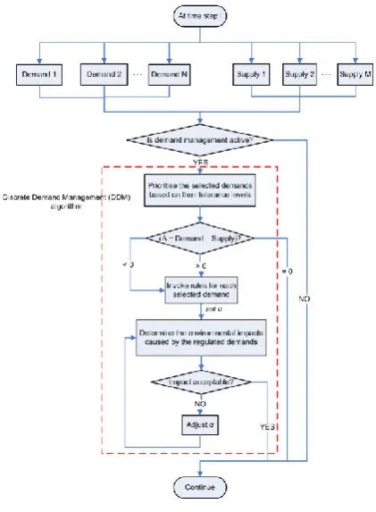
In a simulation context, DDM (Hong, 2009) attempts to minimise the difference between demand and supply at each time step by regulating individual demands while minimising undesirable consequences. The approach minimises the difference, Δ, between the total demand and total supply for a given energy form at any time t.
(1)
where α is a control factor (0-1) that allows the switching of demand over time, P is power (W),
[image:2.595.74.285.378.665.2]spl and dmd refer to supply and demand respectively, and n and m are the total number of supply and demand entities respectively.
Figure 1: DDM algorithm.
With reference to the process flowchart shown in Figure 1, at each time step a search is made to determine what combination of demand management actions will best maximise the match between demand and supply (i.e. minimise equation (1)). The outcome is then assessed in terms of the use impacts of such
actions. Where acceptable, the action is imposed, otherwise it is withheld: e.g. where the proposed action is to down-regulate the heating system but in a manner that would result in unacceptable internal temperatures then α would be reset to zero to withhold the action. Within the process, demands may be defined as not controllable and controllable demands may be prioritised based on tolerance levels (high, medium and low) and subjected to invocation rules, and control may be implemented as on/off or modulated. At any given time, demand management is invoked where total demand exceeds total supply. After acceptable control actions have been applied, the total demand is recalculated through the bottom-up approach, equation (1) revisited, and the process iterated. In this way, the minimum action is applied to achieve an exact or better demand/supply match. Where the total demand is less than the available supply, load recovery may be realised by charging storage systems to store the excess energy. The stored energy can be released at times when the available total supply is insufficient to meet the demand.
DDM ALGORITHM IMPLEMENTATION
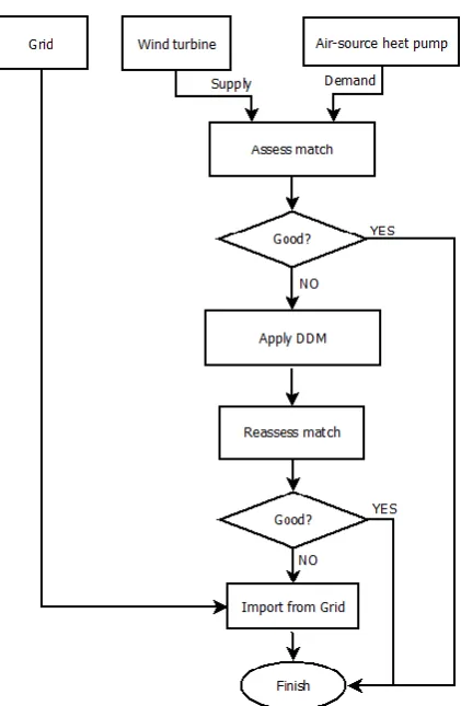
The DDM algorithm is able to assess the potential of demand management approaches and quantify their impact upon the environmental conditions inside a building. Where heating systems are the target, the aim is to utilise the thermal capacity associated with the construction along with the flexibility inherent in occupant thermal comfort preferences to adjust the energy demand pattern to accommodate the prevailing supply. In this way the load profile is reshaped in a manner that creates a match with local intermittent energy supply systems.
with the ESP-r solver to ensure that any disallowed DSM action is not perpetuated over time. The outcome from the process of Figure 2 is an adjusted demand profile that corresponds to the best possible demand/supply match along with information that describes any (acceptable) departure from optimum environmental conditions because of the load manipulation.
Figure 2: DDM as integrated within MERIT and ESP-r.
DDM ANALYSIS OF AN AIR-SOURCE
HEAT PUMP APPLIED TO DIFFERENT
TYPES OF BUILDINGS
The following arbitrary example is included to demonstrate the operation of the DDM modelling approach and the effectiveness of the method. The objective is to assess the potential of DDM, when applied to an air source heat pump used to heat a small office block, to enhance the utilisation of local renewable electricity generation. Both lightweight and heavyweight construction cases are considered. Figure 3 summarises the appraisal process, which relates to a Proven 6.5 kW wind turbine operating cooperatively with the public electricity supply.
Figure 3: Appraising the impact of discreet demand management applied to an air source heat pump.
The simulations are carried out for a weather condition representative of Glasgow under typical winter conditions. The simulation outputs are presented here for a principal zone within the office (Figure 4): an L-shape zone containing five external wall surfaces, three doors, and two windows one on the south facing wall, the other on the east facing wall. For the lightweight construction case, the average U-values are 0.715 W/m2K for the external walls and 2.243 W/m2K for the windows. For the heavyweight case, the wall U-value is changed to 0.239W/m2∙K.
[image:3.595.312.523.64.387.2]
Figure 4: Case study model. the
[image:3.595.313.519.596.735.2]requirements could be down- or up-regulated by manipulating the upper and lower heating set-points:
Rule 1: if θz ≥ θs(h), then θs = θs(h) & α = 0, i.e. switch off heating system;
Rule 2: if θz ≥ θs(l), then θs = θs(l) & α = 1, i.e. switch on heating system;
Rule 3: if θs(l) < θz < θs(h) and Pspl < Pdmd, then
θs = θs(l) & α = 0;
Rule 4: if θs(l) < θz < θs(h) and Pspl ≥ Pdmd, then
θs = θs(h) & α = 1.
where θ is temperature (°C), z and s refer to zone and set-point temperatures respectively, and l and h refer to low and high respectively.
Imposition of these rules allow the demand to be manipulated by shedding heating demand where possible and by widening the set-point range to ‘bank’ available renewable power as long as the space temperature remains below the upper set-point.
[image:4.595.309.523.189.388.2]Three scenarios were set up to investigate the impact of the DDM algorithm upon the building’s energy performance and resulting environmental conditions. The parameter values for each scenario are given in Table 1.
Table 1: Scenario parameters.
The ‘reference’ scenario makes use of an ideal controller to maintain the zone temperature at a constant 21C during the occupied period. For the rest of the time, the heating system is switched off.
The ‘low tolerance’ scenario represents the case when the temperature within the zone is allowed to deviate one degree higher or lower than the above temperature set-point.
The ‘high tolerance’ scenario implies that a higher degree of flexibility (±3C) in the zone temperature is acceptable.
For the ‘low tolerance’ and ‘high tolerance’ scenarios, DDM control is applied during the occupied period only and it is assumed that the system is supplied by a wind turbine, with public supply network backup.
Performance impact before and after applying DDM
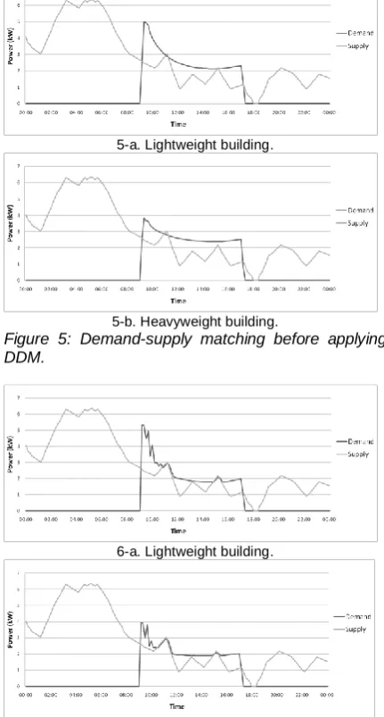
Figures 5-a, 6-a, and 7-a show the simulated heating load and the wind turbine supply profiles for the lightweight construction case. Figures 5-b, 6-5-b, and 7-b show the corresponding results for the heavyweight case.
5-a. Lightweight building.
5-b. Heavyweight building.
Figure 5: Demand-supply matching before applying DDM.
6-a. Lightweight building.
6-b. Heavyweight building.
Figure 6: Demand-supply matching after DDM for the low tolerance case.
7-a. Lightweight building. θs(l) θs(h)
Reference case 21 21 grid connection
ideal basic controller assigned during the occupied period and free floating for the rest.
Case 1 (low tolerance) 20 22
DDM assigned during the occupied period and free floating for the rest.
Case 2 (high tolerance) 18 24
DDM assigned during the occupied period and free floating for the rest. Zone setting points, θs
(o
C)
Scenario Supply side system Buidling control settings
[image:4.595.307.523.200.602.2] [image:4.595.76.281.438.562.2]7-b. Heavyweight building.
Figure 7: Demand-supply matching after DDM algorithm for the high tolerance case.
[image:5.595.69.285.67.173.2]The DDM algorithm can alter the demand profile to follow the pattern generated by the intermittent renewable source. The heavyweight building performs better than the lightweight building in terms of the match with the intermittent supply: because of the higher thermal mass, the peak load is lower. It is evident that the demand/supply match is improved when the demand is greater than the supply, especially in the high tolerance case. Table 2 gives typical simulation outputs: the match between the wind turbine supply and the heating-related electrical demand; the energy utilised from the available wind resource; and the energy imported from the grid. These data show that while the DDM rules result in an increased total energy demand, the same rules can also improve the utilisation of the renewable energy supply and thereby reduce grid energy imports. For this particular example, DDM applied to heating control increases the renewable energy utilisation by 18.9% for the low tolerance case and 15.6% for the high tolerance case. Overall, there was a 56% reduction in the electricity imported from the grid when the set-point temperature was allowed to vary from 1C to 3C.
Table 2: Total energy of demand, direct RE utilisation, and grid importation for each scenario.
Indoor environmental impact before and after applying DDM
In the previous section only the energy impacts were considered. Here the related impact on the indoor environment is quantified.
i) Temperature variation
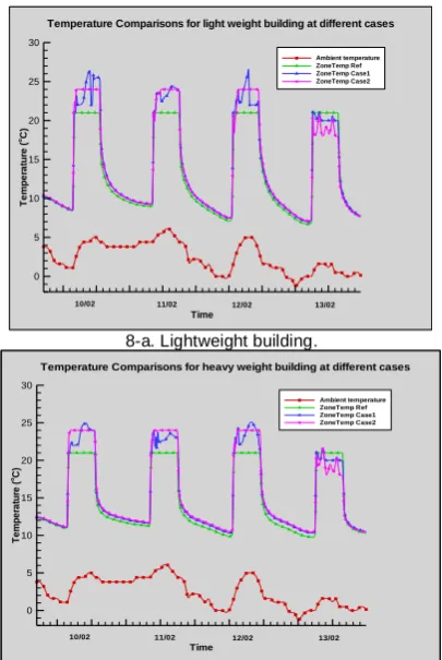
8-a. Lightweight building.
8-b. Heavyweight building. Figure 8: Indoor temperature profiles.
Figure 8 shows the temperature profiles within the office space under the different DDM actions. For the times when there is sufficient energy supply from the renewable system, the zonal temperature in both the lightweight and heavyweight cases under the influence of the DDM is higher than it is when using a a non-DDM controller. Conversely, when energy availability is low, the zonal temperature in both the lightweight and heavyweight cases under the operation of the DDM controller is lower. Another interesting finding when DDM control is active is that when the energy supply/demand is matched, the indoor temperature fluctuation is higher for the lightweight case; while, for the period when demand is greater than supply, higher temperature variations is observed for the heavyweight case.
[image:5.595.315.518.68.371.2]ii) Thermal comfort
Table 3: Comfort index results for different cases.
Average occupant comfort metrics – Predicted Mean Vote (PMV) and Percentage Persons
Light-weight building Heavy-weight building Light-weight building Heavy-weight building Light-weight building Heavy-weight building
Reference Case 471.8 475 / / 471.8 475
Case 1 (low tolerance)
Case 2
(high tolerance) 545.6 565.4 526.1 557 19.5 8.4 Import form grid
(kWh)
560.8 560.2 516.4 533.1 44.5 27.2 Total demand
(kWh)
Direct RE utilised (kWh) Scenario Time T e m p e ra tu re ( oC ) 0 5 10 15 20 25 30 Ambient temperature ZoneTemp Ref ZoneTemp Case1 ZoneTemp Case2 13/02
10/02 11/02 12/02
Temperature Comparisons for light weight building at different cases
Time T e m p e ra tu re ( oC ) 0 5 10 15 20 25 30 Ambient temperature ZoneTemp Ref ZoneTemp Case1 ZoneTemp Case2 13/02
10/02 11/02 12/02
Temperature Comparisons for heavy weight building at different cases
Light-weight building Heavy-weight building Light-weight building Heavy-weight building
Reference Case -0.75 -0.72 18.85% 17.45%
Case 1 (low tolerance)
Case 2
(high tolerance) -0.55 -0.49 15.76% 13.19%
-0.53 -0.52 14.58% 13.23%
Scenario
[image:5.595.69.288.539.597.2] [image:5.595.309.516.656.732.2]Dissatisfied (PPD) – during the occupied period (9:00 to 17:00) are given in Table 3. These two metrics relate to "the difference between the internal heat production and the heat loss to the actual environment for a person kept at the comfort values for skin temperature and sweat production at the actual activity level" (Fanger, 1972). Through introducing the temperature flexibility within the zone and aided with a small proportion of secure electrical power supply from the electrical supply network, the thermal comfort index can be maintained within the range of acceptable comfort.
CONCLUSIONS
This paper has described recent developments of the DDM concept as a means to improve the match between heterogeneous demands and supplies. The approach takes into account the impact on building performance via explicit simulation. An arbitrary example has been given to demonstrate the influence of DDM in enhanced utilisation of local renewable energy sources. It involves an air-source heat pump system powered by a wind turbine with back-up from the public supply network. Two construction types (heavyweight and lightweight) were considered and two levels of DDM were applied corresponding to low and high user tolerance cases. The results show that DDM can alter the demand profile to one that coincides more favourably with an intermittent renewable supply. Generally, the greater the flexibility of demand, the more renewable energy that can be utilised directly, hence reducing the demand placed on the public supply network.
Thus DDM can make a positive contribution to the realisation of future highly distributed energy systems. Future research will focus on the deployment of this DDM approach to seamlessly couple the micro-generation-based energy system with multi-zone buildings, or multiple distributed buildings comprising a community. This would provide more realistic and accurate outcomes to quantify the DDM potential at various levels during the design stage.
ACKNOWLEDGMENT
The authors would like to thank the UK EPSRC for their support for the research project of the Highly Distributed Energy Future under the SuperGen programme.
REFERENCES
Chambers, A., Hamilton, S., and Schnoor, B. 2001. Distributed Generation: A Nontechnical Guide. Tulsa, OK: PennWell.
Charles River Associates 2005. Primer on Demand-Side Management with an Emphasis on Price-Responsive Programs. Report prepared for The World Bank, Washington, DC, CRA No. D06090, available online: http://www.worldbank.org. Dulleck, U. and Kaufmann, S. 2004. Do
customer information programs reduce household electricity demand? – the Irish program. Energy Policy, 32 (2004), pp. 1025-1032.
ESRU 2010a. ESP-r System Version 11.10 Building Performance Simulation Environment. University of Strathclyde, Glasgow, UK. Available:
http://www.esru.strath.ac.uk/Programs/ESP-r.htm.
ESRU 2010b. MERIT Version 3.13. University of Strathclyde, Glasgow, UK. Available:
http://www.esru.strath.ac.uk/Programs/Merit. htm.
Fanger, P.O. 1972. Thermal comfort analysis and applications in environmental engineering. New York: McGraw-Hill. Hong, J. 2009. The Development,
Implementation, and Application of a Demand Side Management and Control Algorithm for Integrated Micro-generation within the Built Environment. PhD Thesis. University of Strathclyde, Glasgow, UK.
Jenkins, N., Allan, R., Crossley, P., Kirschen, D., and Strbac, G. 2000. Embedded Generation. London, UK: IEE.
Kupzog, F. and Roesener, C. 2007. A closer look on load management. in INDIN 2007 - 5th IEEE International Conference on Industrial Informatics, Vienna, Austria, pp. 899-904.
Lopes, J., Hatziargyriou, N., Mutale, J., Djapic, P., and Jenkins, N. 2007. Integrating distributed generation into electric power systems: A review of drivers, challenges and opportunities. Electric Power Systems Research, vol. 77, no. 9, pp. 1189-1203. Williams, E. D. and Matthews, H. S. 2007.