Measurement-based analysis of the dynamic performance of microgrids using system identification techniques

(1)

This paper is a postprint of a paper submitted to and accepted for publication in IET Generation, Transmission and Distribution, and is subject to Institution of Engineering and Technology Copyright. The copy of record is available at IET Digital Library, or http://dx.doi.org/10.1049/iet-gtd.2014.0555

1

Measurement-based Analysis of the Dynamic Performance of

Microgrids using System Identification Techniques

Panagiotis N. Papadopoulos1_{, Theofilos A. Papadopoulos}1_{, Paul Crolla}2_{, Andrew J.}

Roscoe2_{, Grigoris K. Papagiannis}1_{, Graeme M. Burt}2

1_{Power Systems Laboratory, Dept. of Electrical & Computer Engineering,} Aristotle University of Thessaloniki, P.O. Box 486, GR-54124 Thessaloniki, GREECE

Tel: +302310996388, Fax: +302310996302, e-mail: [email protected]

2_{Institute for Energy and Environment, Department of Electronic and Electrical} Engineering, University of Strathclyde

Tel: +4401415482951, Fax: +4401415485872 e-mail: [email protected]

Abstract

The dynamic performance of microgrids is of crucial importance, due to the increased complexity introduced by the combined effect of inverter interfaced and rotating distributed generation. This paper presents a methodology for the investigation of the dynamic behavior of microgrids based on measurements using Prony analysis and state-space black-box modeling techniques. Both methods are compared and evaluated using real operating conditions data obtained by a laboratory microgrid system. The recorded responses and the calculated system eigenvalues are used to analyze the system dynamics and interactions among the distributed generation units. The proposed methodology can be applied to any real-world microgrid configuration, taking advantage of the future smart grid technologies and features.

Keywords

(2)

2

1 Introduction

The increasing penetration of distributed generation (DG) is changing the topology of the traditional power systems. The power flow is becoming bi-directional in low voltage (LV) and medium voltage (MV) networks and microgrids (MGs) are being formed, operating within the distribution networks or in islanded mode [1], [2]. A MG may contain multiple types of DG units, storage devices, and loads each either directly connected or inverter interfaced. Additionally, for each distributed energy resource (DER) conceptually different controls may apply [3]. The integration of the above MG technologies modifies the dynamic behaviour of conventional power systems and therefore, proper analysis tools need to be developed [4].

To ensure the secure and reliable, coordination of different DERs and maximize the penetration of renewable energy sources, the MG dynamic performance as well as the interactions between the DERs must be comprehensively investigated and evaluated under different operating conditions. Especially in MGs, the system stability is very significant, due to the increased complexity introduced by the various components and the lack of a main energy source during islanded operation [3].

(3)

3 dynamic models of parts or of the whole MG as individual controlled entities [25]. The model parameters are directly extracted from measurements without prior knowledge of the exact MG features and structure. However, system identification methods are applied in MGs only on simulation data [23]-[27]. Therefore, the need to ensure the validity of the results from application of system identification methods on real measurement data from MGs is crucial. Moreover, in most cases only the active (P) and reactive power (Q) are analysed, while the voltage (V), the current (I) and the frequency (f) are neglected.

The scope of this paper is to investigate the dynamic performance of MGs, as well as the interactions between DG units using real measurement data. For this purpose two different system identification methods are used and their performance is compared and evaluated. The first method is based on Prony analysis combined with nonlinear least square optimization, while the second on Prediction Error Method (PEM). Furthermore, a comprehensive methodology and general guidelines to develop robust black-box models from measurements are proposed in order to estimate accurately the system eigenvalues and examine the dynamics of all MG system variables, i.e. P, Q, V, I, f. The measured dynamic responses are recorded in a laboratory-scale MG test facility at the University of Strathclyde [28].

2 System Identification techniques for black-box modeling

In this section the theoretical formulation of the two examined system identification methods is presented along with the proposed modeling guidelines and the generalised black-box modelling methodology using real measurement data.

2.1 Prony method

(4)

4 2

1

ˆ( ) i cos( )

n t

i i i

i

y t Ae  t





  

where y tˆ( ) is the fitted response and _i, _i and  _i  _i j_i are the amplitude, phase and eigenvalues, respectively, whereas _i, _i are the corresponding angular frequency and the damping factor [4].

Assuming that the sampling interval is Ts, (1) is transformed to the z-domain as

in (2) [21].

1

ˆ ˆ n k

s i i

i

y k y kT B z



   

   



 

where iTs i

z e .

The n equations of (2) are expressed in matrix form as:

0 0 0

1 2 ₁

1 1 1

2

1 2

1 1 1

1 2 0 1 1 n n

N N N _n

n

y

z z z _B

y B

z z z

B

z  z  z  _{y N}

 _{ }    _ _{ } _{ } _  _{   } _    _{  } _ _{ } _  _{   } _  _{   } _  _{  }_ _ _ _ __   _ _ __     

The characteristic polynomial F(z) with

z

_i as its roots is defined [21]:

 







1 2 0



1 2

1

n

n n n

n i

i

F z z z z a z  a z  a z





       

where the unknown coefficients a_i are identified from the measurement set. The steps to obtain a Prony solution are summarized as follows [21]:

Step 1) Assemble selected data and construct a discrete time prediction model as defined in (5). Several linear solvers can be used for the solution of (5) [20].

1

2

0 1 2 0

1 0 1 1

1 2 3 1 n

y n y n y n y _a

y n y n y n y a

a

y N y N y N y N n

 _ _  _ _ _ _ _{ }                   _ _  _ _ _ _ _{ }                                         _ _  _ _{ } _ _ _         _   _       

Step 2) The roots of the characteristic polynomial of (4) are calculated using the solution of (5), after the a_i coefficients have been identified.

Step 3) The roots of the previous step are associated with the system eigenvalues

i

(5)

5 The efficiency of Prony analysis is limited in case of using distorted measurement data in order to develop low order models. Therefore, nonlinear least square optimization is additionally applied in discrete time form on the measured responses to identify with higher accuracy the unknown parameters of (1) [23], [29]. The proposed procedure is a two-step approach, where first the initial values of the set of parameters

, , , ]

[Ai   i i i



 are determined following steps 1 to 3 of Prony analysis described above. Results from Prony analysis are also used to determine boundaries values of each parameter, following the empirical rules of [29]. Next, nonlinear least square optimization is applied and the parameter set  is adjusted successively in order to match the estimated to the measured response by minimizing the objective function J of (6). Parameters of set  take values in the range set by the corresponding boundaries defined from the previous step.



     

k| y k y kˆ |  6a

 

2

1

|

N i

J  k 





 6b

where 

 

k| is the prediction error (PE), N is the total number of samples and y k

 

,

 

ˆ

y k are the measured and the estimated responses in discrete-time form.

2.2 Prediction Error Method (PEM)

The state space representation of a discrete-time linear model is described as follows:

k+1 k k wk

x = Ax +Bu

 (7)

k k k vk

y =Cx +Du

 (8)

where all matrices are defined at discrete time instant k and

x

_k is the state vector, 1

M

k R

u

_  _and L1

k R

y

_ _{are the input and output vectors, respectively. The unobserved} vector signals

w

_k_RK1_and L1

k R

(6)

6 algorithm [31], [32] and then converted in continuous time form using (9).

 

ln

s

i j i

=

z Ti



(9)

Prediction error methods (PEMs) are a broad family of identification methods that can be applied to arbitrary model parameterization and resemble to the maximum likelihood method [31]. PEMs are iterative methods, where a sequence of past input-output data up to time N-1 _ZN _[ (0), (0),..., (_y _u _{y N}_1), (_{u N}_1)]_{are used to predict the} next one-step output of (8). The general predictor model is defined in (10) in terms of a finite-dimensional parameter vector θ:



1



ˆ( , ) k ,

y k  f Z   (10)

The estimation of θ is performed by minimizing the PE between the predicted outputs ˆ( , )

y k  and the measured outputs ( )y k by means of:

1

argmin ( , N)

N VN Z

   (11)

1

0 1

( , N) N ( ( , ))

N k

k

V Z w k

N  

 



  (12)

Function is a properly chosen criterion, such as the Maximum Likelihood or the Least Square criterion. In this case the two criteria are equivalent and equal to

 

_{  }2

, since the selected systems that are shown next are Single Input Single Output (SISO) [33].

The weighting factor w_k defines how the PE ( , ) t between the measured and the estimated outputs is weighted at specific frequencies [33]. The PEM algorithm incorporated in MATLAB uses a full parameterization of the state space model combined with regularization, with an initial estimation value obtained by the N4SID subspace method [33]. A significant advantage of PEMs is that they can be applied to a wide variety of model structures, providing the best possible results for a given model structure (minimal covariance matrix) [33].

2.3 Black-box modelling methodology

(7)

7 dynamics, as well as to avoid round-off errors [22]. Using the above assumptions the MG system can be assumed linear. The recorded system responses cover the whole transient period as well as the steady-states prior to and after the disturbance with a sufficient sampling rate (2 ms). Therefore, the dynamic responses contain all system mode frequencies typically present in power systems [22], [34]. The length of the time window selected for the identification of the eigenvalues for both methods starts with the initiation of the disturbance and ends right after the oscillations stop.

In most studies the system dynamics are investigated using only the P and Q system variables [23]-[27], while more specifically in Prony analysis only P is modeled [18]-[23]. However, in this paper a modular structure with five computationally decoupled SISO systems is presented, handling not only P and Q variables but also V, I and f recorded at the PCC as well as at the point of connection of the different DG units. Therefore, only the system variables of interest are selected depending on the type of the study performed, e.g. only the frequency or the voltage are used in frequency or voltage stability studies. Although the adopted SISO subsystems are computationally decoupled from each other, all system interactions and coupling between system variables, e.g. f - P or V - Q are included indeed in the respective subsystems. The dynamics of each subsystem are represented by the corresponding eigenvalues that are directly identified from real measured dynamic responses, containing all interactions.

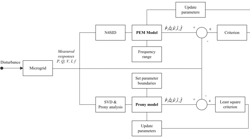
Black-box models are implemented using both Prony and PEM following the corresponding procedure illustrated concisely in Fig. 1. Considering the model order selection for each system variable, an initial estimation is obtained using N4SID for the PEM, while for the Prony method Singular Value Decomposition (SVD) is adopted [31]. Τhe final order for each method is determined individually by further trial and error, in order to achieve the best possible fit. Note that the performance of the PEM is significantly improved by selecting the weighting factors of (12) to emphasize the requirement for a good fit in the frequency range of interest. For this purpose the fast fourier transform (FFT) is applied to the corresponding dynamic responses. Respectively in the proposed Prony method, the FFT is also used for the initial estimation of the frequency parameter as well as to define the corresponding boundaries during the nonlinear-least square procedure [29].

(8)

This paper is a postprint of a paper submitted to and accepted for publication in IET Generation, Transmission and Distribution, and is subject to Institution of Engineering and Technology Copyright. The copy of record is available at IET Digital Library, or http://dx.doi.org/10.1049/iet-gtd.2014.0555 8 (13).

   





 





2 2 1 2 1 ˆ | 1 100 ˆ N d i N d d i

y k y k

R

y k y

                     



(13)

where y_d is the mean value of the measured response. The R2 for all the examined cases in this paper is around 90%.

The proposed methodology is summarized in the following steps:

Step 1) An internal disturbance appears in the MG system, e.g. a load increase. Step 2) The dynamic responses of P, Q, V, I, and f are recorded at the PCC

and the connection point of the DG units.

Step 3) Prony and PEM system identification techniques are applied to the recorded dynamic responses of each system variable.

Step 4) The system eigenvalues involved in the MG dynamics are calculated. Step 5) The developed black-box models are used to analyze and simulate the

dynamic performance of the DG units and the MG.

Microgrid Disturbance PEM Model Prony model SVD & Prony analysis Set parameter boundaries Measured responses P, Q, V, I, f

ˆ ˆ ˆ_{, , , ,}ˆ ˆ

P Q V I f +

-Criterion ε

Update parameters

+ - _{Least square}

criterion ε Update parameters ˆ ˆ ˆ, , , ,ˆ ˆ

P Q V I f

[image:8.595.85.509.410.642.2]

Frequency range N4SID

Fig. 1. Black-box model modelling methodology.

(9)

9 data sets in order to implement a generalized formulation. However, this drawback can be overcome in smart grids with the use of phasor measurement units (PMUs) based on global position system (GPS) and the aid of communication systems [35], making feasible the implementation of online black-box methods for the study of MG dynamics. Additionally, the application of system identification techniques to different types of dynamic responses in a given MG topology can be used as historical data to create databases for offline simulations [29].

3 System Under Study

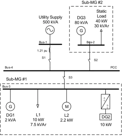
The test facility is a 400-V, three-phase, 50-Hz, laboratory-scale MG with power capacity 100-kVA. The MG configuration is presented in Fig. 2 and is composed of sub-MGs #1 and #2, including directly connected and inverter interfaced DG units as well as a combination of static and dynamic loads. The MG can operate in either grid-connected or islanded mode, using the tie switch S1. A 1.21 per-unit (p.u.) inductance emulates a weak interconnection with the grid, reducing significantly the short circuit capability of the main grid.

DG1 2 kVA

L1 10 kW 7.5 kVAr

DG2

A C D C

G M

Sub-MG #1

10 kW

Bus-3

G

Bus-4

DG3 80 kVA

Static Load 40 kW 30 kVAr Utility Supply

500 kVA

Bus-1 Bus-2

Sub-MG #2

L2 2.2 kW

1.21 pu

S2

PCC S1

[image:9.595.98.339.451.724.2]

S3

(10)

10

3.1 Sub-MG #1

Sub-MG #1 consists of a 2 kVA synchronous generator (DG1), a 10 kVA inverter-interfaced unit (DG2), a 10 kW/7.5 kVAr load bank (L1) and a 2.2 kW, 0.87 lagging asynchronous machine (L2). The synchronous generator is driven by a dc motor emulating a fast-response prime mover. The inverter primary energy source is a dc power supply with constant voltage. Both DG1 and DG2 follow a frequency-active power (f-P), voltage-reactive power (V-Q) droop control scheme, providing frequency and voltage support to the MG. In this study, the asynchronous machine is used only as a motor with controllable torque.

3.2 Sub-MG #2

Sub-MG #2 consists of an 80 kVA synchronous generator (DG3) directly connected to the PCC and of a 40 kW/30 kVAr load bank (L3). The synchronous generator is driven by a dc motor representing a slow-response prime mover. The control scheme followed is an f-P, V-Q droop control and the generator can only operate in islanded mode, supporting the voltage and frequency at the common bus due to its larger nominal power output.

3.3 Experimental setup

The dynamic responses of P, Q, V, I and f are recorded at every MG node. Three test cases (TCs) are conducted for both grid-connected and islanded mode of operation. The TCs are designed to investigate the interactions among DG units in different MG configurations and the influence of droop-controlled DG units.

 TC1: DG1 and L1 are connected, supplying 1 kW/0.75 kVAr and consuming 5kW/2.4 kVAr, respectively.

 TC2: DG2 and L1 are connected, supplying 5 kW/3.75 kVAr and consuming 5kW/2.4 kVAr, respectively.

(11)

11 In all TCs the MG system is subjected to a disturbance, caused by a 40% increase of L1. For all the results presented in the following sections, a positive sign in the active/reactive power and the current variables corresponds to the case that the MG is consuming power from the main grid in grid-connected mode or from Sub-MG#2 in islanded mode.

4 Grid-connected mode of operation

The grid-connected mode of operation is examined for the three TCs, while Sub-MG #1 is connected to a ―weak‖ utility supply grid using the 1.21 pu inductor.

4.1 Eigenvalue analysis

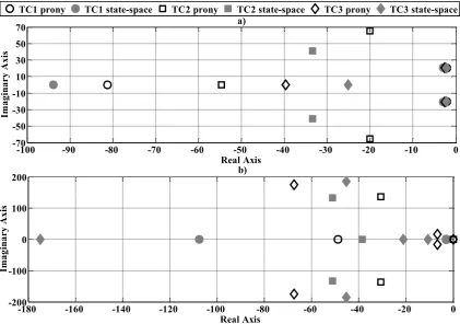
In Fig. 3a and 3b the eigenvalues identified from the active and reactive power responses, respectively, are presented in the complex-plane. Real eigenvalues correspond to exponential decaying modes, while conjugate complex to oscillatory modes. The eigenvalues located close to the imaginary axis present a small exponential decay, thus have a dominant influence on the system response after a disturbance [3], [34]. The eigenvalues of the oscillatory modes of V, I and f are summarized in Table 1. In Table 2 the eigenvalues corresponding to the oscillatory modes, as well as the extracted Prony term Ak of all system components, are analyzed for the generalized TC3

where all DG units are connected to the MG.

(12)

12

-180 -160 -140 -120 -100 -80 -60 -40 -20 0

-200 -100 0 100 200

Real Axis

Im

ag

ina

ry

A

xi

s

b)

TC1 prony TC1 state-space TC2 prony TC2 state-space TC3 prony TC3 state-space

-100 -90 -80 -70 -60 -50 -40 -30 -20 -10 0

-70 -50 -30 -10 10 30 50 70

Real Axis

Im

ag

ina

ry

A

xi

s

[image:12.595.99.521.85.381.2]

a)

Fig. 3. Eigenvalues in the complex plane for the a) Active power b) Reactive power.

Table 1 Eigenvalues for voltage, current and frequency for all cases

V I F

TC1 Prony -10.89±0.22i -1.74±20.82i -6.89±15.57i/ -1.92±19.47i State-space -3.70±1.72i -1.67±20.74i -2.66±18.55i/ -7.33±36.36i TC2 Prony -28.05±35.59i -29.99±150.9i -10.29±21.79i

State-space -0.4±45.91i -34.93±126.8i -10.39±22.83i TC3 Prony -4.73±7.90i/

-24.77±42.63i

-2.60±20.93i -4.38±19i State-space -2.07±13.43i -2.34±21.17i -6.15±18.66i/

[image:12.595.113.482.450.612.2]

(13)

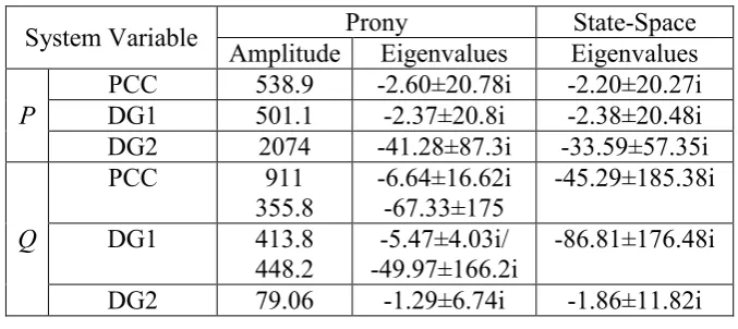
[image:13.595.128.467.103.254.2]

13 Table 2 Prony terms and eigenvalues for TC3

System Variable Prony State-Space

Amplitude Eigenvalues Eigenvalues P

PCC 538.9 -2.60±20.78i -2.20±20.27i DG1 501.1 -2.37±20.8i -2.38±20.48i DG2 2074 -41.28±87.3i -33.59±57.35i

Q

PCC 911

355.8 -6.64±16.62i -67.33±175 -45.29±185.38i

DG1 413.8

448.2 -49.97±166.2i -5.47±4.03i/ -86.81±176.48i DG2 79.06 -1.29±6.74i -1.86±11.82i

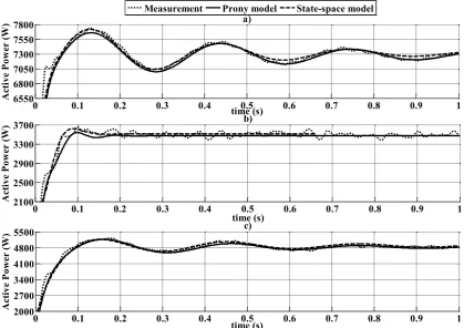
4.2 Active power response

(14)

14

0 0.1 0.2 0.3 0.4 0.5 0.6 0.7 0.8 0.9 1

6550 6800 7050 7300 7550

7800 a)

time (s)

A

cti

ve

P

ow

er

(W)

0 0.1 0.2 0.3 0.4 0.5 0.6 0.7 0.8 0.9 1

2100 2500 2900 3300

3700 b)

time (s)

A

cti

ve

P

ow

er

(W)

0 0.1 0.2 0.3 0.4 0.5 0.6 0.7 0.8 0.9 1

2000 2700 3400 4100 4800

5500 c)

time (s)

A

cti

ve

P

ow

er

(W)

[image:14.595.100.520.86.382.2]

Measurement Prony model State-space model

(15)

15

0 0.1 0.2 0.3 0.4 0.5 0.6 0.7 0.8 0.9 1

0 1000 2000 3000 4000 5000

6000 a)

time (s)

A

cti

ve

P

ow

er

(W)

0 0.1 0.2 0.3 0.4 0.5 0.6 0.7 0.8 0.9 1

0 1000 2000 3000

4000 b)

time (s)

R

ea

cti

ve

P

ow

er

(V

ar)

DG1 DG2

[image:15.595.102.515.85.392.2]

DG1 DG2

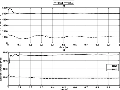
Fig. 5. Measurements of DG1 and DG2 for TC3 a) active and b) reactive power.

(16)

16

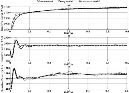
4.3 Reactive power response

In Fig. 6 measurement and simulation results are compared for the reactive power at the PCC, while in Fig. 5b the DG1 and DG2 recorded reactive power responses for TC3 are presented. In all TCs the voltage drop at Bus-4, due to the influence of the load L1 step change causes DG units to balance the MG reactive power, according to the V – Q droop characteristics.

In TC1 the adjusted reactive power share after the disturbance is obtained after some ms, due to the delayed response of the automatic voltage regulator (AVR) of DG1. The fast oscillations in the first ms of the MG reactive power dynamic response in TC2 and ΤC3 are attributed to the influence of the V-Q control of DG2 as analyzed in Fig. 5b [16].

0 0.1 0.2 0.3 0.4 0.5 0.6

1500 1900 2300 2700

3100 a)

time (s)

R

ea

cti

ve

P

ow

er

(V

A

r)

0 0.1 0.2 0.3 0.4 0.5 0.6

500 1000 1500 2000

2500 b)

time (s)

R

ea

cti

ve

P

ow

er

(V

A

r)

0 0.1 0.2 0.3 0.4 0.5 0.6

400 600 800 1000

1200 c)

time (s)

R

ea

cti

ve

P

ow

er

(V

A

r)

[image:16.595.98.522.334.637.2]

Fig. 6. Measurement and simulation results for the reactive power at the PCC for a) TC1, b) TC2, c) TC3.

(17)

17 first one is related to the fast reaction time of DG2 with a frequency at 7.4 Hz, while the second is at 1.26 Hz and is due to the delayed response of DG1. Therefore, the two system modes in TC3 are not the superposition of TC1 and TC2 modes, due to the reactive power participation share of DG units and the interactions between the DG2 V -Q control and the DG1 AVR.

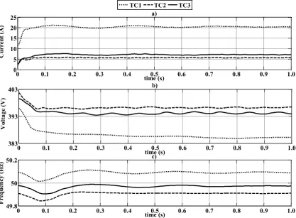
4.4 Voltage, current and frequency responses

In Fig. 7 the current, voltage and frequency measurements at the PCC are illustrated for all TCs. It can be generally observed that the current presents a similar response to the active power, whereas the voltage to the reactive power, resulting also to similar eigenvalues as analyzed in Tables 1 and 2. Only in TC2 the current is influenced by the reactive power change of DG2, since a high frequency mode of 18 Hz is involved in the dynamic response.

0 0.1 0.2 0.3 0.4 0.5 0.6 0.7 0.8 0.9 1.0

0 5 10 15 20 25

time (s)

C

urrent

(A

)

a)

TC1 TC2 TC3

0 0.1 0.2 0.3 0.4 0.5 0.6 0.7 0.8 0.9 1.0

383 393 403

time (s)

V

ol

ta

ge

(V

)

b)

0 0.1 0.2 0.3 0.4 0.5 0.6 0.7 0.8 0.9 1.0

49.8 50 50.2

time (s)

F

requency

(Hz)

[image:17.595.102.520.379.686.2]

c)

(18)

18 Voltage responses generally present a time-delayed form with negligible oscillations. In such cases it is harder to identify the system eigenvalues, using the two modeling techniques and extract the corresponding model parameters. In TC2 and TC3 the fast dynamics of DG2 cause small oscillations, similar to those in the reactive power responses introducing an eigenvalue at 7.3 Hz with high damping.

The oscillatory nature of the MG frequency response as well as the relatively large deviations from the nominal frequency of 50 Hz at the PCC is due to the weak interconnection of the MG with the main grid. In TC1 and TC3 the frequency oscillation is mainly caused by DG1, while in TC3 higher damping is observed, due to the fast reaction of the inverter-interfaced DG2 as shown in Table 2. In TC2 the oscillation exhibits significantly high damping with the absence of rotating machines.

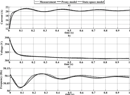
In Fig. 8 the laboratory measurements for TC1 of I, V and f are compared with the corresponding simulation results, using the two modeling techniques. Also in this case, negligible differences are recorded, validating the accuracy of the developed models.

0 0.1 0.2 0.3 0.4 0.5 0.6 0.7 0.8 0.9 1

12 14 16 18 20

22 a)

time (s)

C

urrent

(A

)

0 0.1 0.2 0.3 0.4 0.5 0.6 0.7 0.8 0.9 1

384 389 394

398 b)

time (s)

V

ol

ta

ge

(V

)

0 0.1 0.2 0.3 0.4 0.5 0.6 0.7 0.8 0.9 1

50 50.05 50.1

50.15 c)

time (s)

F

requency

(Hz)

[image:18.595.100.515.398.702.2]

(19)

19

5 Islanded mode of operation

In islanded mode Sub-MG #2 is also connected, providing voltage and frequency support to Sub-MG #1. All TCs are examined and Sub-MG #1 is modeled using both black-box methods.

5.1 Eigenvalue analysis

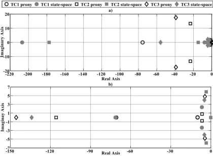
The identified eigenvalues for the active and reactive power are presented in Fig. 9a and 9b, respectively. Compared to the grid-connected mode, conjugate complex eigenvalues of lower frequency are observed, due to the predominant influence of the large mass DG3 in the MG power share. The eigenvalues identified by both techniques present small differences for all TCs.

-220 -200 -180 -160 -140 -120 -100 -80 -60 -40 -20 0

-20 -10 0 10

20 a)

Real Axis

Im

ag

ina

ry

A

xi

s

TC1 prony TC1 state-space TC2 prony TC2 state-space TC3 prony TC3 state-space

-150-7 -120 -90 -60 -30 0

-5 -3 -1 1 3 5

7 b)

Real Axis

Im

ag

ina

y

A

xi

[image:19.595.98.519.389.697.2]

s

(20)

20

5.2 Dynamic responses analysis

In this scenario the system frequency and voltage at Bus-4 is significantly affected by the step-change of L1. All DG units adjust their active and reactive power, according to the corresponding droop characteristics.

In Fig. 10 measurement and simulation results of the active power at Bus-4 of Sub-MG #1 are compared. In all TCs an oscillation of 0.25 Hz is observed, caused by the electromechanical mode of DG3. Compared to the grid-connected scenario the dominant system mode presents lower frequency and higher damping, due to the larger inertia and the slower prime mover of DG3. DG2 has no inertia, thus is influenced by the system frequency variation, shown in Fig. 11, according to the f-P droop. On the contrary in TC1, a smaller oscillation is observed, since DG1 is less sensitive to system variations compared to DG2. Measured dynamic responses of the individual DG units are recorded in Fig. 12 for TC3, where the oscillations of DG2 are highlighted.

0 0.5 1 1.5 2 2.5

4500 5500 6500

7500 a)

time (s)

A

cti

ve

P

ow

er

(W)

0 0.5 1 1.5 2 2.5

0 1500 3000

4500 b)

time (s)

A

cti

ve

P

ow

er

(W)

0 0.5 1 1.5 2 2.5

1000 2500 4000

5500 c)

time (s)

A

cti

ve

P

ow

er

(W)

[image:20.595.99.522.395.696.2]

(21)

21

0 0.5 1 1.5 2 2.5

0 5 10 15 20 25 time (sec) C urrent (A ) a)

TC1 TC2 TC3

0 0.5 1 1.5 2 2.5

375 390 405 time (sec) V ol ta ge (V ) b)

0 0.5 1 1.5 2 2.5

[image:21.595.103.521.87.386.2]

49.8 49.9 50 50.1 time (sec) F requen cy (Hz) c)

Fig. 11. Measurements at the PCC for all TCs for a) current, b) voltage c) frequency.

0 0.5 1 1.5 2 2.5

500 2500 4500 6500 time (s) A cti ve P ow er (W) a) DG1 DG2

0 0.5 1 1.5 2 2.5

(22)

22 Fig. 12. Measurements of DG1 and DG2 for TC3 a) Active power b) Reactive power.

In all TCs the reactive power dynamic response of the MG at the PCC is oscillatory with relative small amplitude as shown in Fig. 13. In TC1 the dominating frequency is around 0.35 Hz, due to the slow reaction of the AVRs of DG1 and DG3. In TC2 and TC3 the dominant frequency is at 0.9 Hz with lower damping, due to the interactions of the droop-controlled DG2 and the rotating DG units. Comparing the reactive power responses and the eigenvalues of Sub-MG #2 with the corresponding of the grid-connected case, it is shown that in TC2 and TC3, the high frequency oscillations in the initial few ms of the responses, associated with DG2, are practically eliminated in the case of the islanded operation. This is attributed to the reactive power share participation of DG3 [16].

0 0.1 0.2 0.3 0.4 0.5 0.6 0.7 0.8

1500 2500

3500 a)

time (s)

R

ea

cti

ve

P

ow

er

(V

ar)

0 0.1 0.2 0.3 0.4 0.5 0.6 0.7 0.8

-500 0 500 1000

1500 b)

time (s)

R

ea

cti

ve

P

ow

er

(V

ar)

0 0.1 0.2 0.3 0.4 0.5 0.6 0.7 0.8

0 500 1000

1500 c)

time (s)

R

ea

cti

ve

P

ow

er

(V

ar)

Fig. 13. Measurement and simulation results for reactive power at the PCC for a) TC1, b) TC2, c) TC3.

[image:22.595.101.522.339.630.2]

(23)

23 supported in TC2 and TC3, where DG2 is present. The frequency dynamics include eigenvalues with higher damping, lower frequency around 0.25 Hz and larger amplitude compared to the grid-connected case. This is attributed to DG3 with large inertia and slow prime mover response.

6 Discussion

Based on the conducted test cases the following conclusions can be summarized: Microgrid operation:

The eigenfrequencies of the involved modes during disturbances vary from 0.3 Hz to 20 Hz corresponding to the electromechanical and controller modes of DG units as well as to interactions among them. The system eigenvalues are influenced by the DG properties (type, capacity, control scheme) and the MG configuration (mode of operation and participation of rotating and droop-controlled units).

The electromechanical modes of rotating DG units are the dominating oscillatory modes of the system and influence significantly the small-signal dynamics of MG configurations in islanded and weak grid conditions. Droop-controlled DG units have an insignificant impact on the eigenfrequencies of these modes. The dynamic performance of DG units is significantly influenced by the

interactions with other DG units or with the grid. Therefore, the MG system eigenvalues are not always the result of superposition of the corresponding DG unit eigenvalues in case of stand-alone operation.

In LV MGs current and voltage responses are more or less similar to the active and reactive power responses, respectively.

During weak grid operation, droop controlled DG units contribute mainly to voltage regulation and the reactive power share of MGs, according to their corresponding droop characteristics. Their penetration results in higher damping and lower oscillation amplitude in the active power response as well as in higher damping in the reactive power oscillations.

(24)

24 influence the MG dynamic responses for both the active and reactive power, since their behavior depends strongly on the frequency and voltage variation at the MG buses. The penetration of droop controlled units may amplify oscillations in grids including DG synchronous generators.

Black-box modelling:

The accuracy of both identification methods can be significantly improved with the aid of an initial rough estimate of the frequencies contained in the dynamic responses, especially when dealing with real measurement data. More specifically, in Prony method an initial value of the frequency parameter as well as the corresponding boundaries are set during nonlinear least square optimization, while for the PEM proper weighting of the data during the criterion minimization process is used.

Both methods can lead to accurate results for all system variables under real world operating conditions and can represent the dynamic behavior of the MG as well as of the individual DG units, especially in cases presenting a pronounced oscillatory form.

In cases where small or no oscillations are observed, approximate models can be developed using only exponential decaying terms with zero frequency.

In several TCs Prony analysis is more accurate than state-space modeling. This is attributed to the use of proper boundaries and initial estimations of each parameter separately in contradiction to the PEM method. Moreover, it provides the opportunity to develop empirical rules to further improve the method performance.

The Ak parameters of the Prony method provide direct information of the

oscillations amplitude. This can be used for the investigation of the influence of different parameters on the MG response.

7 Conclusions

(25)

25 paper. The proposed methodology can be used in the development of accurate microgrid black-box models.

Prony analysis and the PEM techniques are applied on the recorded dynamic responses and the results are compared. The developed models perform well and can be useful tools for the dynamic analysis of a whole microgrid or of parts of it as individual aggregated entities. These aggregated models can be accessible by the Distribution System Operator and can be used for efficient wide-area control, wide-area monitoring and ancillary service provision studies. By embedding the models developed with the proposed methodology within the Distribution System Operator‘s management system it will allow the operator to make use of the microgrid and possibly encourage the development of more MGs within their network area.

Several experimental test cases are investigated at a laboratory scale MG and from the analysis of the dynamic responses significant remarks considering the microgrid small-signal dynamics are concluded. The major contributions include the investigation of the interactions between inverter interfaced and rotating generators, the identification and analysis of the involved system modes from measurements and the comparison of the MG performance in grid-connected and islanded operation.

8 Acknowledgements

The work of T. A. Papadopoulos is supported by the ‗ΙΚΥ Fellowships of excellence for postgraduate studies in Greece – Siemens program‘.

Laboratory measurements were conducted in the frame of the Distributed Energy Resources Research Infrastructure (DERri) project under the European FP7 Programme.

8. References

[1] Chowdhury S., Chowdhury S.P., and Crossley P.: ―Microgrids and Active Distribution Networks‖ (IET, 2009).

(26)

26 [3] Katiraei F., Iravani M.R.: "Power Management Strategies for a Microgrid With Multiple Distributed Generation Units", IEEE Trans. Power Syst., 21, (4), pp.1821-1831, Nov. 2006.

[4] Crow M., Gibbard M., Messina A., Pierre J., Sanchez-Gasca J., Trudnowski D., Vowles D.: ―Identification of Electromechanical Modes in Power Systems‖, IEEE Technical Report, Task Force on Identification of Electrmechanical modes, June 2012.

[5] Annakkage U.D., Nair N.K.C., Liang Y., Gole A.M., Dinavahi V., Gustavsen B., Noda T., Ghasemi H., Monti A., Matar M., Iravani R., Martinez J.A.: "Dynamic System Equivalents: A Survey of Available Techniques", IEEE Trans. on Power Delivery, 27, (1), pp.411-420, Jan. 2012.

[6] Etemadi A.H., Davison E.J., Iravani R.: "A Decentralized Robust Control Strategy for Multi-DER Microgrids—Part I: Fundamental Concepts", IEEE Trans. on Power Delivery, 27, (4), pp.1843-1853, Oct. 2012.

[7] Katiraei F., Iravani M.R., Lehn P.W.: "Small-signal dynamic model of a micro-grid including conventional and electronically interfaced distributed resources", IET Generation, Transmission & Distribution, 1, (3), pp.369-378, May 2007. [8] Zhixin M., Domijan A., Lingling F., "Investigation of MGs with Both Inverter

Interfaced and Direct AC-Connected Distributed Energy Resources", IEEE Trans. Power Del., 26, (3), pp.1634-1642, July 2011.

[9] Trudnowski D.I.: "Order reduction of large-scale linear oscillatory system models", IEEE Trans. on Power Systems, 9, (1), pp.451-458, Feb 1994.

[10] Ishchenko A., Myrzik J.M.A., Kling W.L.: "Dynamic equivalencing of distribution networks with dispersed generation using Hankel norm approximation", IET Generation, Transmission Distribution, 1, (5), pp.818-825, September 2007.

[11] Price W.W, Hargrave A.W., Hurysz B.J., Chow J.H., Hirsch P.M.: "Large-scale system testing of a power system dynamic equivalencing program", IEEE Trans. on Power Systems, 13, (3), pp.768-774, Aug 1998.

(27)

27 [13] Hauer J.F.: "Application of Prony analysis to the determination of modal content and equivalent models for measured power system response", IEEE Trans. on Power Systems, 6, (3), pp.1062-1068, Aug 1991.

[14] Zhao B., Zhang X., Chen J.: "Integrated Microgrid Laboratory System", IEEE Trans. on Power Systems, 27, (4), pp.2175-2185, Nov. 2012.

[15] Salehi V., Mohamed A., Mazloomzadeh A., Mohammed O.A., "Laboratory-Based Smart Power System, Part II: Control, Monitoring, and Protection", IEEE Trans. Smart Grid, 3, (3), pp.1405-1417, Sept. 2012.

[16] Lasseter R.H., Eto J.H., Schenkman B., Stevens J., Vollkommer H., Klapp D., Linton E., Hurtado H., Roy J.: "CERTS Microgrid Laboratory Test Bed", IEEE Trans. Power Del., 26, (1), pp.325,332, Jan. 2011

[17] Hatziargyriou N., Asano H., Iravani R., Marnay C.: "Microgrids", IEEE Power Energy Mag., July/August, 2007.

[18] Barklund E., Pogaku N., Prodanovic M., Hernandez-Aramburo C., Green T.C.: "Energy Management in Autonomous MG Using Stability-Constrained Droop Control of Inverters", IEEE Trans. Power Electron., 23, (5), pp.2346-2352, Sept. 2008.

[19] Sanchez-Gasca J.J., Chow J.H.: "Performance comparison of three identification methods for the analysis of electromechanical oscillations", IEEE Trans. Power Systems, 14, (3), pp.995-1002, Aug. 1999.

[20] Zhou N., Pierre J., Trudnowski D.: "Some considerations in using Prony analysis to estimate electromechanical modes", Proc. Power and Energy Society General Meeting (PES), 2013 IEEE.

[21] Hauer J.F., Demeure C.J., Sharf L.L.: "Initial results in Prony analysis of power system response signals," IEEE Trans. on Power Systems, 5, (1), pp.80-89, Feb. 1990.

[22] Grund C.E., Paserba J.J., Hauer J.F., Nilsson S.: "Comparison of Prony and Eigenanalysis for Power System Control Design", IEEE Trans. on Power Systems, 8, (3), pp.964-971, August 1993.

(28)

28 [24] Papadopoulos P.N., Papadopoulos T.A., Papagiannis G.K.: "Dynamic modeling of a microgrid using smart grid technologies", UPEC 2012, London 4-7 Sept. 2012.

[25] Zali S.M., Milanovic J.V.: "Generic Model of Active Distribution Network for Large Power System Stability Studies", IEEE Trans. on Power Systems, 28, (3), pp. 3126-3133, Aug 2013.

[26] Resende F.O., Pecas Lopes J.A.: "Development of Dynamic Equivalents for MicroGrids using System Identification Theory", PowerTech, 2007, Lausanne, pp.1033-1038, July 2007.

[27] Feng X., Lubosny Z., Bialek J.W., "Identification based Dynamic Equivalencing," Proc. Power Tech, 2007 IEEE Lausanne.

[28] Roscoe A.J., Mackay A., Burt G.M., McDonald J.R.: "Architecture of a Network-in-the-Loop Environment for Characterizing AC Power-System Behavior", IEEE Trans. on Industrial Electronics, 57, (4), pp.1245-1253, April 2010.

[29] Papadopoulos P.N., Papadopoulos T.A., Crolla P., Roscoe A.J., Papagiannis G.K., Burt G.M.: "Black-box dynamic equivalent model for microgrids using measurement data", IET Gener., Trans. and Distrib., 8, (5), pp.851-861, May 2014.

[30] Favoreel W., De Moor B., Van Overschee P.: "Subspace state space system identification for industrial processes", Journal of Process Control, 10, pp. 149-155, 2000.

[31] Katayama T.: ―Subspace Methods for System Identification‖ (Springer, 2005). [32] Matlab R2011b http://www.mathworks.com.

[33] Ljung L.: ―System Identification Theory for the User‖, (Prentice Hall, 1999). [34] Elgerd O.I: ―Electric Energy Systems Theory: An Introduction‖ (McGraw-Hill,

1982).