Towards semi-automated non-destructive evaluation

Towards semi-automated non-destructive evaluation

L Fradkin1, V Zernov1,6, G Elston2, R Taneja2, I Bell3, D Lines4, J Wharrie4 and P Fitzgerald5

1

Sound Mathematics Ltd., 11 Mulberry Close, Cambridge, CB4 2AS, UK 2

Doosan Power Systems, Porterfield Road, Renfrew, PA4 8DJ, UK 3

National Instruments , Measurement House, Newbury Business Park, London Road, Newbury, Berkshire RG14 2PZ, UK

4

Diagnostic Sonar Ltd., Baird Road, Kirkton Campus, Livingston, EH54 7BX, UK 5

LabVIEW Certified Developer, Lewkenors Mill, Denham, Bury St Edmunds, Suffolk IP29 5EF, UK

6

Now at SmartOdds, 53-79 Highgate Road, London, NW5 1TL, UK

E-mail: l.fradkin@soundmathematics.com

Abstract. A demonstrator has been developed showing feasibility of semi-automatic characterisation of large planar flaws in steel using ultrasonic transducer arrays. The unit is based on a real-time ultrasonic imager deploying National Instruments hardware and software, is connected to an IMASONIC linear phased array containing 128 elements and incorporates a novel flaw characterisation algorithm, which is a model-based variant of Total Focusing Method, taking into account undulations in inspection surface. It has been shown to process RF data collected in immersion reasonably fast and be capable of detecting and characterising with reasonable accuracy large planar defects.

1.Introduction

We have addressed a high level, long-term challenge of the ultimate deployment of an innovative ultrasonic unit for flaw characterisation and interpretation that would lead to cost effective and reliable semi-automatic NDE (Non-Destructive Evaluation). No existing instrumentation offers real-time automatic flaw diagnostics and at present, while some phased array ultrasonic inspections themselves are automated the data collected are still being interpreted by human inspectors, leading to variability in reporting [1]. The most surprising outcome of the above study conducted by TWI (The Welding Institute) is that inspectors experience the greatest difficulty when characterising large planar cracks. Probably less surprisingly the most difficult cracks to identify are those normal to inspection surface.

In this study we work with real data collected in immersion, with the main source of error being undulations in the inspecion surface and show that a simple modification of a TFM (Total Focusing Method) supported by a simple model of a large planar crack can produce a reasonably fast algorithm for crack characterisation. The paper is organised as follows: in the next section we describe the demonstrator developed, experiments conducted and signals collected, we then report our findings and compare our images to the ones obtained using the standard FMC (Full Matrix Capture) algorithm as implemented in our demonstrator. We finish by discussing our results and future plans.

2.Description of the demonstrator and experiments

History and issues surrounding real-time ultrasonic array imaging using FMC and TFM have been described in many publications, see e.g. [7]. The demonstrator built during this study took full advantage of flexible and scalable acquisition hardware modules, thus reducing instrument cost and size. The acquisition time has been reduced by introducing significant levels of parallelism, using standardised PC-based modular hardware. Generic hardware (the FlexRIO family from National Instruments) based on FPGAs (Field Programmable Gate Arrays) has been combined with customized analogue hardware (NI-5752) to produce a 32 channel 12-bit 50 MSPS acquisition module with digitally controlled swept gain. The multiplexer used on transmit has been implemented as a stackable PCB module to multiplex to a 128 element IMASONIC linear transducer array. The module is able to multiplex the 32 receive channels over all 128 elements. FPGAs handle the high data rates from many parallel channels. While existing techniques take two or more seconds to process each image the new architecture achieves acquisition at 20Hz and higher. The IMASONIC array employed in the study has had the elementary pitch of 0.8 mm, inter element space of 0.25 mm and total active length of 102.15 mm. All elements have been employed to transmit simultaneously the signal with the centre frequency of 2 MHz ±10%, the bandwidth ≥ 55 % and pulse duration < 1500 ns (see figure 1).

The specimen used in experiments was a steel block, 30 mm thick, 200 mm wide, 350 mm long, containing four surface-breaking notches and four embedded ones, some tilted some – non-tilted. The full description of the notches is given in table 1. The experiments have been performed in immersion, with the water temperature of 22.00C and water path standoff distance of about 13 mm. The geometry of the experiment is presented in figure 2.

0 10 20 30 40

Figure 2. Schematic of the experiments

The present version of the demonstrator generates data in the form of .png files. These are used to be processed by either standard or modified TFM and stored for future use. A LabVIEW application has been written that can read these .png files and convert them into a Full Matrix [Fijk, i, j = 1,2,…128, k = 1,…, Alen] of A-scans, where the first index denotes the transmitter, the second – the receiver and the third – the time sample. Alen has been normally chosen to be 800 to deal with pulse trains 800

µsec long. The standard FM produces images of specimen sections utilising the intensity function

=

∑

(x _x (1)

where h_tx,rx(t) is the Hilbert transform (analytic representation) of the signal A_tx,rx(t) and t_tx,x,rx

is the time of travel from a transmitter tx to receiver rx through a node x=(x,z). The nodes are evenly spaced throughout each section. The Hilbert transform is defined by

τ

τ

τ

π

u v p t A H

∫

= 1 . . ( )

) )( (

provided the integral exists as a principal value. The summation in (1) is carried out for each possible transmitter–receiver pair in the array. Even when the input signal is a perfect delta function rather than the pulse presented in figure 1 the intensity function can produce misleading results: In the worst case scenario, if the transducer array is in direct contact with the specimen, only one transducer element is used in both transmit and receive and there is only one point scatterer, all specimen points lying on an arc of a circular wave front radiated by this element and reaching the scatterer are characterised by the same time of arrival and therefore are assigned the same intensity. Inspecting in immersion and involving more than one element reduces this possibility but does not eliminate it. The fact that different portions of a pulse arrive at different moments in time increases the probability of false indications.

z, mm

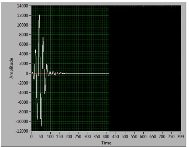
Figure 3. A typical pulse train recorded at array element 17 (elements are numbered left to right). The first pulse – echo from the upper surface of the specimen of the pulse transmitted by element 17, the second pulse – surface echo of the pulse transmitted by element 1, the third pulse – backwall echo of the pulse transmitted by element 17. The backwall echo of the pulse transmitted by element 1 arrives later or not at all. Time is measured in microseconds.

3. Semi-automatic crack characterisation

As mentioned at the end of the previous section, applying the intensity function (1) different points on the grid that surrounds a scattering point can pick up different portions of the same scattered pulse. This can lead to a smudged image of the scatterer and maybe, to an error in its positioning. The brightest point in the image can be close to, but not necessarily on, the scatterer. For this reason, Wiener deconvolution has been tried to identify an impulse response function but it has produced no discernibly superior results and is not employed in the final algorithm. However the above considerations have been combined with a priori knowledge that the notches are linear features a few wave lengths in extent and thus, when in TOFD configurations, can produce two bright spots around edge diffraction points. The resulting LabVIEW application first combines image and signal processing algorithms to implement a model-based modification of TFM to identify such spots. It then joins their centres by a straight segment to characterise the defect in terms of its orientation (in degrees) with respect to the inspection surface, extent (in mm) and depth (in mm), that is, the shortest distance from a defect end to a specimen’s surface (the inspection surface or else the backwall). It has been found that the diffraction points are best identified by utilising the intensity function (1) with the summation carried over a portion of the array, which we call a fictitious aperture, rather than the whole array. This is due to the fact that when the full aperture is used the specular reflections from the inspection surface can be very intense and mask diffraction signals from defect edges.

A

m

pl

it

(a) (b)

(c)

Figure 4. Comparison of images of a non-tilted embedded defect, imaged from the notched block side (notch 3 in table 1). (a) - the image obtained with a standard TFM algorithm, (b) – the image obtained with a model-based version of TFM, (c) - the resulting report. (a) demonstrates that in this case the straightforward application of TFM produces no defect image. (b) presents in black and white two diffraction spots identified using the model-based version of TFM. The report in (c) contains the profile of the specimen’s upper surface and the defect image suggested by the diffraction spots as well as the associated defect parameters (bottom right) and parameters of the image processing filters that have been used to generate (b) (top right).

A typical pulse train is presented in figure 3 and a typical report - in figure 4. Typical results are summarised in table 1. Extensive data analysis has shown that to achieve successful defect characterisation several aspects of the problem require attention:

wave speeds in water and steel, they lead to significant change of the ray paths – see figure 5, where different approximations of the upper surface are used, a polynomial and a constant, respectively. Numerical experimentation has been used to establish the range of interpolation parameters within which the sensitivity of defect images to these parameters is at its lowest. In future interpolation will be effected using cubic splines.

2. As table 1 illustrates, there are issues with characterising surface-breaking defects when imaging form the notched surface. Analysis has shown that these are due to failing to detect the diffraction points lying in the inspection surface. Similar difficulties face human inspectors. However, our results suggest that identification can be improved by employing image processing filters which incorporate a priori knowledge of properties of scattered signals.

3. Occasionally we see false indications. Therefore all solutions suggested by our application should be presented to a human operator to allow him/her to select those that appear most reasonable.

4. When analysing data pertaining to all studied defects it has been found that the most advantageous length of fictitious aperture is 20 mm. In each case position of this aperture is selected automatically.

Table 1. Comparison of estimated and actual characteristics of notches imaged from either flat or notched side of the test steel block.

Notch no/type/ inspection surface

Estimated/specified extent

Estimated/specified orientation

Estimated/specified Depth

1/embedded/flat 9mm/10 mm 700/700 7mm/5 mm

1/embedded/notched 10 mm/10 mm 700/700 9 mm/5 mm

2/embedded/flat 5 mm /5 mm 700/700 5 mm /5 mm

2/embedded/notched 4 mm/5 mm 700/700 8 mm/5 mm

3/embedded/flat 10mm/10 mm 900/900 3 mm/5 mm

3/embedded/notched 9 mm /10 mm 840/900 6 mm/5 mm

4/embedded/flat 4.5/5 mm 900/900 4.5 mm/5 mm

4/embedded/notched 4 mm/5 mm 900/900 7 mm/5 mm

(a)

(b)

Figure 5. (a) Upper surface profile approximated by a 10th degree Polynomial and resulting raw image. (b) Upper surface profile approximated by a 0th degree polynomial (constant) and resulting raw image.

4. Speed of execution

the other hand, the speed of the LabView implementation of the standard TFM running on our demonstrator matches its speed of data acquisition at 20 Hz or higher. Thus, a significant speed-up of our application could be achieved by re-writing MathScript modules in LabVIEW. An alternative fast version could be written in C.

5. Conclusions

A model-based version of Total Focusing Method has been developed and implemented in LabVIEW for semi-automated characterisation of large isolated planar cracks in stainless steel. The reported feasibility study has shown that simulating configurations which produce diffraction from defect edges usually leads to reliable defect sizing, even though further work is required to study and reduce probability of false indications. The capability of application was demonstrated using a steel block with realistically undulated surfaces and containing four embedded and four surface-breaking relatively large planar notches, some tilted and some non-tilted. It is possible to extend the procedure to other types of defects and geometrical configurations, developing a comprehensive library of generic models for eventual deployment in a portable probe capable of acting as a real-time assistant to an ultrasonic inspector and interpreter.

The proposed solution for semi-automatic characterisation of safety critical defects, which would result in clear and unambiguous reports, could support the existing fleet of nuclear reactors as well as the new build. It could be later spun-out into other industries, such as rail or oil and gas.

Acknowledgments

This project was funded by Technology Strategy Board under their Nuclear R&D Feasibility Studies Program and the authors are indebted to the Board for their imaginative strategies for setting up creative consortia. The authors are also grateful to the TSB monitoring officer Tom Harris for his critical feedback and constant support.

References

[1]

Schneider C and Bird C 2009

Proc

24th – 26th June 2009 Berlin Germany

[2] Champagnat F, Goussard Y and Idier J 1996 IEEE Transactions on Signal Processing 44(12) 2988

[3] Holmes C, Drinkwater B W and Wilcox P D 2008 Ultrasonics 48 636

[4] Hunter A J, Drinkwater B W and Wilcox P D 2008 IEEE Trans Ultrason Ferroelectr Freq Control. 2008 55(11) 2450

[5] Hunter A J, Drinkwater B W and Wilcox P D 2011 IEEE Trans Ultrason Ferroelectr Freq Control 58(2) 414

[6] Marengo E A, Fred K G and Simonetti F 2007 IEEE Transactions On Image Processing 16( 8) 1967