City, University of London Institutional Repository
Citation
:
Castro-Alvaredo, O. and Fring, A. (2000). Renormalization group flow with
unstable particles. Physical Review D (PRD), 63(2), doi: 10.1103/PhysRevD.63.021701
This is the unspecified version of the paper.
This version of the publication may differ from the final published
version.
Permanent repository link:
http://openaccess.city.ac.uk/725/
Link to published version
:
http://dx.doi.org/10.1103/PhysRevD.63.021701
Copyright and reuse:
City Research Online aims to make research
outputs of City, University of London available to a wider audience.
Copyright and Moral Rights remain with the author(s) and/or copyright
holders. URLs from City Research Online may be freely distributed and
linked to.
City Research Online:
http://openaccess.city.ac.uk/
[email protected]
arXiv:hep-th/0008208v2 6 Sep 2000
Renormalization group flow with unstable particles
O.A. Castro-Alvaredo♯and A. Fring⋆
♯Departamento de F´ısica de Part´ıculas, Universidad de Santiago de Compostela, E-15706 Santiago de Compostela, Spain
⋆
Institut f¨ur Theoretische Physik, Freie Universit¨at Berlin, Arnimallee 14, D-14195 Berlin, Germany
(February 1, 2008)
The renormalization group flow of an integrable two di-mensional quantum field theory which contains unstable par-ticles is investigated. The analysis is carried out for the Vira-soro central charge and the conformal dimensions as a func-tion of the renormalizafunc-tion group flow parameter. This allows to identify the corresponding conformal field theories together with their operator content when the unstable particles van-ish from the particle spectrum. The specific model considered is theSU(3)2-homogeneous Sine-Gordon model.
PACS numbers: 11.10Hi, 11.10Kk, 11.30Er, 05.70.Jk
The study of two-dimensional quantum field theories (2D-QFT) has turned out to be a fruitful venture since almost three decades. In particular when exploiting inte-grability many non-perturbative methods have been de-veloped over the years. Besides the challenge to under-stand the underlying mathematical structures and the intriguing physical applications in two dimensions itself, e.g. to describe measurable quantities of carbon nan-otubes [1], the ultimate goal is to extrapolate ones find-ings to higher dimensions. In particular for the cele-brated c-theorem of Zamolodchikov [2], which originally describes the renormalization group trajectory of a func-tion which at the renormalizafunc-tion group fixed point cor-responds to the Virasoro central charge, various coun-terparts have been developed in higher dimensions, e.g. [3].
Fairly recently a class of massive integrable quan-tum field theories, the homogeneous Sine-Gordon models (HSG) [4], has been proposed introducing the feature of possessing unstable particles inside its particle spectrum. Despite the fact that theories containing resonances have been treated before in the context of two-dimensional massive quantum field theories, e.g. [5], the HSG-models are somewhat special since they constitute the first ex-amples of theories which admit a well-defined Lagrangian description. In general the HSG models are associated to integrable perturbations ofG-parafermions of levelk[6], i.e. WZNW-coset theories of the form Gk/U(1)ℓ withℓ
being the rank of a compact Lie groupG. As free param-eters the model containsℓdifferent mass scales andℓ−1 different scales for the resonance parameterσ which en-ter the Breit-Wigner formula [7]. In general an unstable particle of type ˜cis described by complexifying the phys-ical mass of a stable particle by adding a decay width Γc˜,
such that it corresponds to a pole in the S-matrix as a function Mandelstamsats=MR2 = (M˜c−iΓc˜/2)2 (for
a more detailed discussion see e.g. [8]). As mentioned in [8] whenever M˜c ≫Γc˜, the quantity M˜c admits a clear
cut interpretation as the physical mass. However, since this assumption is only required for interpretational rea-sons we will not rely on it. Transforming as usual in this context from s to the rapidity plane and describ-ing the scatterdescrib-ing of two stable particles of typeaand b
with massesma andmb by an S-matrixSab(θ) as
func-tion of the rapidityθ, the resonance pole is situated at
θR=σ−iσ¯. Identifying the real and imaginary parts of
the pole then yields
Mc˜2−
Γ2 ˜
c
4 =m
2
a+m2b+ 2mambcoshσcos ¯σ (1)
M˜cΓ˜c= 2mambsinh|σ|sin ¯σ . (2)
Eliminating the decay width from (1) and (2), we can ex-press the mass of the unstable particlesM˜c in the model
as a function of the masses of the stable particlesma, mb
and the resonance parameterσ. Assumingσto be large this gives
M2 ˜
c ∼
1
2mamb(1 + cos ¯σ)e
|σ|. (3)
One recognizes the occurrence of the variable me|σ|/2,
which was introduced originally in [9] in order to describe massless particles, i.e. one may perform safely the limit
investigate how a particular coset flows to another one. On the other hand, we study in addition the flow of the operator content of one conformal field theory to another one by exploiting the flow provided by the ∆-sum rule of Delfino, Simonetti and Cardy [13].
Denoting byrthe radial distance and byt= lnr2 the
renormalization group parameter, the functionsc(t) and ∆(t) were defined in [2] and [13], respectively, obeying the differential equations
dc(t)
dt =−
3 4e
2t
hΘ(t)Θ(0)i (4)
d∆(t)
dt =
1
hO(0)ie
thΘ(t)O(0)i . (5)
The r.h.s. of these equations involve the two-point cor-relation functions of the trace of the energy-momentum tensor Θ and an operator O, which is a primary field in the sense of [14]. In general these equations are in-tegrated from t = −∞to t =∞ and one consequently compares the difference between the ultraviolet and the infrared fixed points. In order to exhibit the quantitative onset of the mass scale of the unstable particles we inte-grate these equations instead from some finite valuet0to infinity. Restricting our attention to purely massive the-ories we use the fact that for those thethe-ories the infrared central charges are zero, such that
c(r0) = 3 2
∞
Z
r0
dr r3 hΘ(r)Θ(0)i . (6)
Instead of the integral representation (6), thec-function is equivalently expressible in terms of a sum of correla-tors involving also other components of the energy mo-mentum tensor [2]. In deriving (4) these terms have been eliminate by means of the conservation law of the energy momentum tensor. We find (6) most convenient. The flow of c(r0) will surpass various steps: Starting with
r0= 0 the theory will leave its ultraviolet fixed point and at a certain definite value, sayr0=ru, the unstable
par-ticle will become massive such thatc(r0> ru) can be
as-sociated to a different conformal field theory. It appears natural to identify the mass M˜c as the point at which
c(r0) is half the difference between the two coset values ofc. As a consequence of (3) we may relate the masses of the unstable particles at different values of the resonance parameterσ,σ′ and expectM˜
c(ru, σ) =M˜c(r′u, σ′). We
will employ the latter equality evaluated in the form (3) not only as a consistency requirement, but also as a con-firmation of the fact that the renormalization group flow is indeed achieved bym →r0m. Increasing r0 further, the energy scale of the stable particles will eventually be reached at, say at r0 =ra, rb, . . . , rn. Depending on the
relative mass scales between the stable particles these points may coincide. Finally the flow will reach its in-frared fixed pointc(r0=rir) = 0.
Likewise we can integrate equation (5)
∆(r0) =− 1
2hO(0)i
∞
Z
r0
dr r hΘ(r)O(0)i , (7)
which allows to keep track of the manner the opera-tor contents of the various conformal field theories are mapped into each other. We used that all conformal dimensions vanish in the infrared limit. Fortunately, we
havehΘ(r)O(0)i ∼ hO(0)iin many applications such that
the vacuum expectation valuehO(0)icancels often. One should note, however, that (7) is only applicable to those operators for which its two-point correlator with the trace of the energy momentum tensor is non-vanishing, such that one may not be in the position to investigate the flow of the entire operator content by means of (7).
In order to evaluate (6) and (7) we have to compute the two-point correlation functions in some way. In 2D-QFT this is probably most efficiently achieved, by ex-panding them in terms of n-particle form factors, i.e. the matrix elements of some local operatorO(~x) located at the origin between a multiparticle in-state and the vac-uum denoted byh0|O(0)|Vµ1(θ1)Vµ2(θ2). . . Vµn(θn)iin=: FO|µ1...µn
n (θ1, . . . , θn). Here the Vµ(θ) are some
ver-tex operators representing a particle of species µ. Ab-breviating the sum of the on-shell energies as E = Pn
i=1mµicoshθi, one may write
hO(r)O′(0)i=
∞
X
n=1
X
µ1...µn
∞
Z
−∞
dθ1. . . dθn
n!(2π)n e
−r E (8)
×FO|µ1...µn
n (θ1, . . . , θn)
FO′|µ1...µn
n (θ1, . . . , θn)
∗
.
Using this expansion we replace the correlation functions in the expression of the c-function c(r0) and the scaled conformal dimension ∆(r0) and perform the r integra-tions thereafter. Thus we obtain
c(r0) = 3
∞
X
n=1
X
µ1...µn
∞
Z
−∞
dθ1. . . dθn
n!(2π)n e
−r0E (9)
×
F
Θ|µ1...µn
n (θ1, . . . , θn)
2(6 + 6r0E+ 3r2
0E2+r03E3)
2E4
and
∆(r0) =−
∞
X
n=1
X
µ1...µn
∞
Z
−∞
dθ1. . . dθn
n!(2π)n
(1 +r0E)e−r0E 2E2 (10)
×FΘ|µ1...µn
n (θ1, . . . , θn)
FO|µ1...µn
n (θ1, . . . , θn)
∗
.
We will now analyze (9), (10) and (3) for the SU(3)2
-HSG model. This model contains only two self-conjugate solitons which we denote by “+”, “−” and one unsta-ble particle, which call ˜u. The corresponding scatter-ing matrix was found [16] to be S±± = −1, S±∓(θ) =
may not be formed. Note that for the corresponding value of ¯σ=π/2 and arbitraryσthe conditionM˜u≫Γu˜
is not fulfilled. However, as indicated above this condi-tion only helps for a clearer identificacondi-tion of the mass parameter. For the HSG-models this condition starts to hold when the level is large, which indicates that in these type of models this interpretation is in fact a semi-classical one.
A huge class of form factors corresponding to vari-ous operators related to this model were constructed in [15,12]. Labelling an operator by four quantum numbers
µ, ν, τ, τ′ the general n-particle solution reads
FO µ,ν
τ,τ′|M
+
M−
2s+τ,2t+τ′ (θ1, . . . , θn) =H
Oµ,ν
τ,τ′|M
+
M− 2s+τ,2t+τ′ detA
µ,ν
2s+τ,2t+τ′ σ2+s+τ
s−t+τ
−1−ν
2 σ−
2t+τ′
1+τ−τ′
−µ
2 −tY
i<j
ˆ
Fµiµj(θ
ij). (11)
We used here a particular ordering by starting with 2s+τ
particles of the typeµ= + followed by 2s+τ′particles of
the typeµ=−, collected in the setsM± ={±, . . . ,±}.
Once these expressions are known, all other form factors related to it by permutations of the particles may be con-structed trivially by exploiting Watson’s equations [17], see [15,12] for details concerning the HSG-models. The functions ˆFµiµj for all combinations of theµ’s are
ˆ
F±±(θ) =−i/2 tanhθ
2exp(∓θ/2) (12) ˆ
F±∓(θ) = 21 4e
iπ(1∓1)±θ
4 − G π− R∞ 0 dt t sin2
((iπ−θ∓σ) t
2π) sinhtcosht/2 , (13)
with G = 0.91597. . . being the Catalan constant. The (t+s)×(t+s)-matrix
Aµ,ν2s+τ,2t+τ′
ij=
σ+
2(j−i)+µ, 1≤i≤t
ˆ
σ−2(j−i)+2t+ν , t < i≤s+t (14)
has as its entries elementary symmetric polynomials (see e.g. [18] for properties) depending on different sets of vari-ables. We use the notationσ± when they depend on the
variable x = expθ associated to the sets M± and ˆσ to
indicate that all variables are multiplied by a factorie−σ.
The overall constant was computed to
HO µ,ν
τ,τ′|M
+
M− 2s+τ,2t+τ′ =i
s(2τ+τ′
+ν+2)2s(2s−2t−τ′
−1+2τ)
×esσ(2t+τ′
)/2HO µ,ν
τ,τ′
τ,2t+τ′, (15)
where the value of HO µ,ν
τ,τ′
τ,2t+τ′ is fixed by the lowest
non-vanishing form factor. In particular we need
F2Θs,2t=σ1(x1, . . . , xn)σ1(x−11, . . . , x−n1)F
O1,1 2,2
2s,2t . (16)
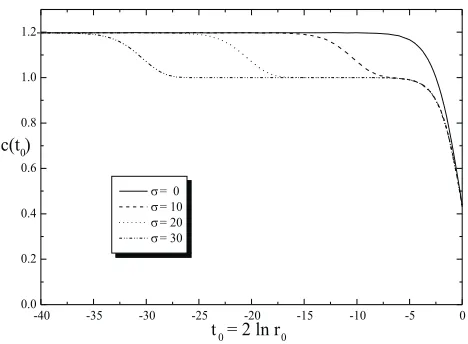
[image:4.612.323.557.54.226.2]Having assembled all the ingredients we can evaluate the expressions (9) and (10). We carry out the integrals by means of a Monte Carlo computation. Forc(r0) we take contributions up to the 4-particle form factor into ac-count and display our results in figure 1.
Figure 1: Renormalization group flow for the Virasoro central chargec(r0) for various values of the resonance parameterσ.
Following the renormalization group flow from the ul-traviolet to the infrared, figure 1 illustrates the flow from theSU(3)2/U(1)2- to theSU(2)2/U(1)⊗SU(2)2/U (1)-coset when the unstable particle becomes massive. This confirms qualitatively the previous observation of the TBA analysis [10]. Here we also want to compare the value of the mass of the unstable particle at different points of the resonance parameter σ and t0. Taking now the mass scales of the stable particles to be the same, i.e. m+ = m− = m, we compute the mass of
the unstable particle according to (3), i.e. Mu˜(tu, σ) ∼
m/√2 exp((|σ|+tu)/2). This means for different values
of the resonance parameter we may still have the same value for the mass of the unstable particle when changing
tu, indeed we find
Mu˜(−30.8,30) =Mu˜(−20.8,20) =M˜u(−10.8,10). (17)
Since the flow between the two cosets is smooth and takes place over some range of t0, we had to select one par-ticular point tu. As already indicated in general, it is
convenient to identify M˜u as the point at which c(t0)
is half the difference between the two coset values of c. It is clear from figure 1, that since the overall shape of the curves between two values of c is identical for dif-ferent values ofσ, any other value in the interval would lead to the same results in comparative considerations. This also means that when evaluating (17) the resulting value 0.47m, which apparently violates the energetically necessary conditionM˜u> ma+mb, should not be taken
too literally since the pointtuis only chosen because it is
easy to fix. Equations (17) confirm our general assertions outlined above.
For the evaluation of the scaled conformal dimension (10) we proceed similarly. For the solutions correspond-ing to the operatorsO00,,00,O
0,1 0,2 and O
1,0
2,0, whose
Figure 2: Renormalization group flow for the conformal di-mension ∆(r0) of the operatorO
0,0
0,0 for various values of the resonance parameterσ.
We observe that the conformal dimension of the op-erator O00,,00 flows to the value 1/8, which is twice the
conformal dimension of the disorder operator µ in the Ising model. The factor 2 is expected from the mentioned coset structure, i.e. we find two copies ofSU(2)2/U(1). The nature of the operator is also anticipated, since by
constructionFO
0,0 0,0|M
+
M−
n of theSU(3)2-HSG model
co-incides precisely withFµ
n of the thermally perturbed Ising
model when one of the setsM± is empty. It is also clear
that we could alternatively obtain (17) from the analysis of ∆(r0).
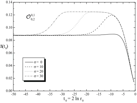
Figure 3: Renormalization group flow for the conformal di-mension ∆(r0) of the operatorO
0,1
0,2 for various values of the resonance parameterσ.
Despite the fact that the explicit expressions for the form factors ofO00,,12 and O
1,0
2,0 differ the values of ∆(r0)
are hardly distinguishable and we therefore omit the plots for the latter case. We also note the previously observed fact [12], that the higher particle contributions for the latter operators are more important than forO00,,00, which
explains the fact that the starting point at the ultraviolet fixed point is not quite 0.1. The operators also flow to the value 1/8, such that the degeneracy of theSU(3)2-HSG
model disappears surjectively when the unstable particles become massive.
In comparison with other methods it would be ex-tremely desirable to elaborate on the precise relation-ship between c(r0) and the finite size scaling function of the thermodynamic Bethe ansatz. Also the relation to the intriguing proposal in [19] of a renormalization group flow between Virasoro characters remains unclar-ified. The analogue of ∆(r0) still needs to be identified in the TBA as well as in the context of [19]. In addition one may pose the question whether there exist higher di-mensional counterparts of the function ∆(r0) in analogy to the results obtained in [3] for c(r0). Concerning the specific status of the HSG-models it remains a challenge to extend the results to other Lie groups [20].
Acknowledgments: A.F. is grateful to the Deutsche
Forschungsgemeinschaft (Sfb288) for financial support. O.A.C. thanks CICYT (AEN99-0589), DGICYT (PB96-0960), and the EC Commission (TMR grant FMRX-CT96-0012) for partial financial support and is also very grateful to the Institut f¨ur theoretische Physik of the Freie Universit¨at for hospitality and for partial financial support. We are grateful to J.L. Miramontes, G. Mus-sardo for useful comments and A. Schilling for discussions on [19].
[1] Special Issue,Physics World,13, 29 (2000). [2] A.B. Zamolodchikov,JETP Lett. 43, 730 (1986). [3] J.L. Cardy, Phys.Lett. B215, 749 (1988); H. Osborn,
Phys.Lett.B222,97 (1989); N.E. Mavromatos, J.L. Mi-ramontes and J.M. Sanchez de Santos,Phys.Rev. D40,
535 (1989); I. Jack and H. Osborn, Nucl.Phys. B343,
647 (1990); G.M. Shore,Phys.Lett.B253,380 (1991); A. Cappelli, J.I. Latorre and X. Vilasis-Cardona,Nucl.Phys.
B376,510 (1992); F. Bastianelli, Phys.Lett. B369,249 (1996); J. Erdmenger and H. Osborn,Nucl.Phys.B483,
431 (1997); S. Forte and J.I. Latorre,Nucl.Phys.B535,
709 (1998); J. Gaite,Phys.Rev. D61,045006 (2000); J. Gaite,On renormalization group irreversible functions in more than two dimensions, hep-th/0005107; A. Cappelli and G. D’Appollonio, Phys.Lett. B487, 87 (2000); D. Anselmi,JHEP6, 42 (2000).
[4] C.R. Fern´andez-Pousa, M.V. Gallas, T.J. Hollowood and J.L. Miramontes, Nucl. Phys. B484, 609 (1997); Q-H. Park, Phys. Lett. B328, 329 (1994); T.J. Hollowood, J.L. Miramontes and Q-H. Park,Nucl. Phys.B445,451 (1995).
[image:5.612.61.294.419.595.2]165 (1979); Al.B. Zamolodchikov, Nucl. Phys. B 358,
524 (1991); M.J. Martins, Phys. Rev. Lett. 69, 2461 (1992); Nucl. Phys. B394, 339 (1993); P. Dorey and F. Ravaninni,Int. J. Mod. Phys. A8,(1993) 873; Nucl. Phys.B406,708 (1993); C. Ahn, G. Delfino and G. Mus-sardo,Phys.Lett.B317,573 (1993); G. Mussardo and S. Penati,Nucl. Phys.B567, 454 (2000).
[6] D. Gepner,Nucl. Phys.B290,[FS20] 10 (1987). [7] G. Breit and E.P. Wigner,Phys. Rev.49,519 (1936). [8] R.J. Eden, P.V. Landshoff, D.I. Olive and J.C.
Polk-inghorne, The analytic S-Matrix (CUP, Cambridge, 1966).
[9] Al.B. Zamolodchikov,Nucl. Phys.B358(1991) 524. [10] O.A. Castro-Alvaredo, A. Fring, C. Korff and J.L.
Mira-montes,Nucl. Phys.B573, 535 (2000).
[11] A.B. Zamolodchikov,Phys. Lett.B253, 391 (1991). [12] O.A. Castro-Alvaredo and A. Fring,Identifying the
Op-erator Content, the Homogeneous Sine-Gordon models,
hep-th/0008044.
[13] G. Delfino, P. Simonetti and J.L. Cardy, Phys. Lett.
B387, 327 (1996).
[14] A.A. Belavin, A.M. Polyakov and A.B. Zamolodchikov,
Nucl. Phys.B241,333 (1984).
[15] O.A. Castro-Alvaredo, A. Fring and C. Korff, Phys. Lett.
B484, 167 (2000).
[16] J.L. Miramontes and C.R. Fern´andez-Pousa,Phys. Lett.
B472, 392 (2000).
[17] P. Weisz,Phys. Lett.B67,179 (1977); M. Karowski and P. Weisz, Nucl. Phys.B139,445 (1978).
[18] I.G. MacDonald,Symmetric Functions and Hall Polyno-mials(Clarendon Press, Oxford, 1979).
[19] O. Foda and Y.-H. Quano, Int.J.Mod.Phys. A12, 1651 (1997); A. Berkovich, B.M. McCoy and A. Schilling,
Physica A228, 33 (1996); L. Chim, J.Math.Phys. 40, 3761 (1999).