Direct occlusion handling for high level image processing algorithms

(1)

Theses Thesis/Dissertation Collections

2-1-2009

Direct occlusion handling for high level image

processing algorithms

Carl Ryan Kelso

Follow this and additional works at:http://scholarworks.rit.edu/theses

This Thesis is brought to you for free and open access by the Thesis/Dissertation Collections at RIT Scholar Works. It has been accepted for inclusion in Theses by an authorized administrator of RIT Scholar Works. For more information, please [email protected].

Recommended Citation

(2)

Level Image Processing Algorithms

by

Carl Ryan Kelso

A Thesis Submitted in Partial Fulfillment of the Requirements for the Degree of

Master of Science in

Computer Engineering

Supervised by

Associate Professor Dr. Juan C. Cockburn Department of Computer Engineering

Kate Gleason College of Engineering Rochester Institute of Technology

Rochester, New York February 2009

Approved by:

Dr. Juan C. Cockburn, Associate Professor

Thesis Advisor, Department of Computer Engineering

Dr. Shanchieh Yang, Associate Professor

Committee Member, Department of Computer Engineering

Dr. Joseph Geigel, Associate Professor

(3)

Rochester Institute of Technology Kate Gleason College of Engineering

Title:

Direct Occlusion Handling for High Level Image Processing Algorithms

I, Carl Ryan Kelso, hereby grant permission to the Wallace Memorial Library to reproduce my thesis in whole or part.

Carl Ryan Kelso

(4)

Dedication

To my parents and my advisors.

(5)

Acknowledgments

I am grateful for the help my sister Catherine provided in the process of writing this work. Her tireless assistance provided not only a connection to the vast body of work in the field of neural science, but also provided much of the polish my document needed. She, and her professors, have proven to

(6)

Abstract

Direct Occlusion Handling for High Level Image Processing Algorithms

Carl Ryan Kelso

Supervising Professor: Dr. Juan C. Cockburn

(7)

List of Tables

2.1 A variety of derivative kernels . . . 20

2.2 The fundamental derivative kernels used by Lindeberg . . . 25

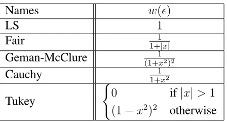
3.1 A variety of M-Estimators . . . 51

4.1 Effect of varying the X-threshold on polygon edge segments. 75

(10)

List of Figures

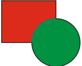
1.1 In the figure above, a green circle is visually in front of a

red rectangle. The dotted edge bordering both is intrinsic to

the circle, but extrinsic to the rectangle. . . 2

1.2 A piece of paper, a hand over it, and the resulting paper

with the simplest shape prediction. Final image modified in

Corel Photopaint 8. . . 4

1.3 A red ball rolls behind a blue pillar. The visible region on

the left shrinks until vanishing completely. In every frame,

the ball is partially visible. Images created in Corel Bryce 5. 7

1.4 A flow chart depicting the system. . . 9

2.1 Demonstration of the presence of a blind spot in human vision. 17

2.2 Demonstration of edge completion in the presence of a blind

spot. . . 18

2.3 Demonstration of curve completion in the presence of a

blind spot. . . 18

2.4 Kanizsa’s triangle. This figure produces the appearance of

a white triangle over three circles. Note the appearance of a

white on white edge at the border of the triangle. There is

no local gradient to hint at its presence. . . 19

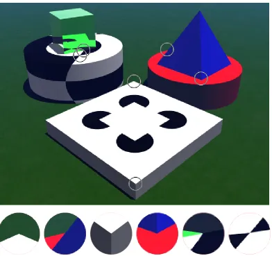
2.5 An image illustrating many of the different possible types

of junctions. From left to right, these are the typical L, T,

Y, followed by a concave Y, A reflective X, and a clear X.

(11)

2.6 A well known optical illusion demonstrating the three

di-mensional bistability of Y-junctions. Are the red regions

squares on top of boxes, below the boxes, or are they

dia-monds? . . . 29

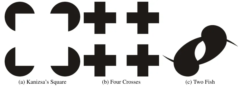
2.7 Images of Kanizsa’s Square (a), the four crosses image (b),

and the spontaneous splitting two fish image (c) described

by Geiger et al.[9]. . . 29

2.8 The relationship between an edge and its detected points. . . 32

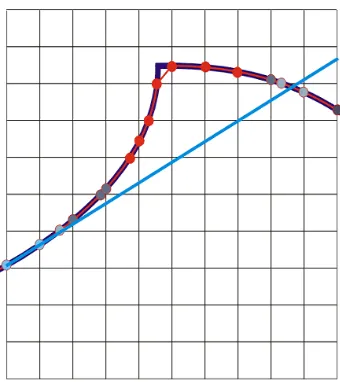
3.1 Demonstration of fit sensitivity across gaps without

cumu-lative minimum thresholding . . . 53

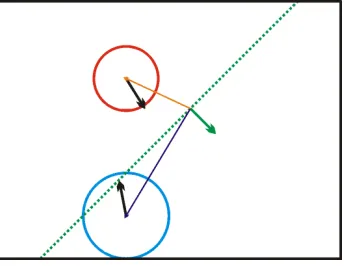
3.2 A small sample BSP space. The green vector is a local root

node. It splits the space into two hemi-planes. In the front

hemi-plane is the blue vector, which has a fit length that

passes the hemi-plane border. The red vector in the back

hemi-plane, on the other hand can safely ignore things in

the front hemi-plane since its fit is shorter than the distance

to the border. . . 56

4.1 The Gaussian test images. Each image varies in standard

deviation of blur from 1 px to 128 px as the image is

tra-versed from top to bottom respectively. . . 61

4.2 Each image is processed using a blur filter with a variance

of 1₂ px. The process without sub-sampling used 16 blurs, while the process with sub-sampling used 8 per sub-sample.

The lower images are vectorized versions of the outputs for

clarity . . . 63

4.3 Each image in this set was blurred 8 times per sub-sample

(12)

4.4 Each image in this set was blurred with a 3 × 3 Gaussian

filter with variance of 1₂px2, and sub-sampled with

re-up-sampling enabled. . . 65

4.5 This looks at the variance around the ideal blur per

sub-sample described by Eaton et al.[7]. The base image is the

quadratically increasing Gaussian step to highlight smaller

scales. . . 66

4.6 This test bank blurs each image to a standard deviation of

2pxbefore sub-sampling with a blur kernel of the specified

variance. . . 67

4.7 A comparison of the edge detector output using

rotation-ally symmetric versus separable blur kernels. Each image is

blurred to a standard deviation of 2 px before sub-sampling . 68

4.8 A comparison of the output produced by three common

tive kernels (and their convolution for second order

deriva-tives) . . . 69

4.9 Five simple convex shapes. From left to right: A square,

pentagon, octagon, dodecagon and circle. From top to

bot-tom: The generated edge with a single vertex (at top for

all except the circle, which is at right), polynomial fits, and

junction closures. . . 71

4.10 A demonstration of the limit of junction detectability in the

estimator. The polygons from left to right are 24, 25, and 26

sided. All junctions are found on the 24 sided figure. The

top right corner is lost on the 25 sided figure. Only seven

junctions are detected in the 26 sided figure, one of which

(13)

4.11 Four simple convex shapes. From left to right: A square,

pentagon, octagon and dodecagon. From top to bottom: The

original image, the extracted edge, the polynomial fits, and

resulting junction closures. . . 73

4.12 A trefoil: a three dimensional knot. Rendered in Corel Bryce 5. . . 74

4.13 The result of varying the X-threshold on fits. . . 75

4.14 The result of varying the W-threshold on fits. . . 76

4.15 The result of varying the G-threshold on fits. . . 76

4.16 The test edge for comparing various M-Estimators. . . 77

4.17 The results of applying each M-Estimator to the test image. The columns from left to right are the results from the Least Squares, Fair, Geman-McClure, Cauchy, and Tukey estima-tors respectively. From top to bottom are the progressive fits to the system, followed by the final fits, and the result-ing completions. . . 78

4.18 The result of varying the W-threshold on fits. The distance between each pair is measured in the length of the side of a square. . . 81

4.19 The result of varying the W-threshold on fits. . . 82

4.20 A demonstration of the system processing splitting figures. . 83

4.21 A demonstration of the system processing complex figures. . 84

4.22 Additional complex figure examples. . . 85

(14)

B.1 Three Gaussian step images used to test the edge detector’s

responsiveness at different scales. The images are designed

to produce a vertical edge down the center of the image. An

ideal edge detector will return an uninterrupted edge at this

location. Two additional edges are expected at the border

(15)

Glossary

A

amodal completions (amodal) When the human visual system com-pletes objects, it may not necessarily create the sensation of a vis-ible edge. If the completion occurs in the behind an occluder, it is referred to as an amodal completion. An example is the percep-tion of completed circles in a Kaniza’s Square. While the edge is not visible, it can be traced., p. 11.

articulated An object composed of many components connected via joints. An example of an articulated object is a skeleton.

B

Binary Spatial Partitioning (BSP) A specific type of spatial indexing system. Binary Spatial Partitioning organizes spatially correlated information by recursively splitting the data in to convex subsets based on an easily calculated metric. Through careful choice of the splitting metric, and balancing, it is possible to reduce search-ing in the space from O(n2) toO(nlogn), p. 39.

blob A localized region of pixels or features derived from an image with similar properties. If these properties are easy to calculate then tracking blobs can be a fast an efficient means of following objects without high level processing., p. 3.

blue-noise Noise which is dominant in high spatial frequencies, but not present in low spatial frequencies., p. 20.

(16)

to tackle the issue. This may take longer than a top down strategy, but can yield better results., p. 1.

C

Canny’s edge detector An edge detector developed in the 1980s which takes raw input data from a typical linear filter based derivative op-erator and performs several non-linear operations to refine edges down to a width of a single pixel., p. 10.

center-surround A receptive field pattern for a neuron. This pattern is typically recognizable by a cluster of inputs surrounded by a second cluster with opposite polarity. This structure is able to recognize the presence of details, which stimulate the inner field without affecting the outer field. The same structure in the eye may connect different colors to the center and the surround re-spectively, allowing most humans to distinguish betwen adjacent hues., p. 15.

Cesaro Equation An equation which relates a curve’s curvature to its arc-length.

Charge Coupled Devices (CCD) A capacitive array originally designed for use as a memory device. They have found application as the image sensors in digital cameras. See also Complementary Metal Oxide Semiconductors., p. 13.

chiasma The point in the brain where information from both eyes is sorted by hemisphere so information from a persons left and right hemispheres of vision can be processed for stereo correlations., p. 15.

(17)

Complementary Metal Oxide Semiconductor (CMOS) A class of digital circuits which uses a capacitive barrier to control the active state of a gate. CMOS circuits tend to be very low power, and have found application as the light sensitive components in certain image sensors. See also Charge Coupled Devices., p. 13.

Compute Unified Device Architecture (CUDA) A C-like program-ming language developed by NVIDIA to extend access to the functionality of their highly parallelized floating point GPU hard-ware., p. 9.

D

Difference of Gaussian (DoG) The difference of two gaussian kernels with different variances. The DoG operator can be used as an approximation of the LoG operator. It is the basis for the SIFT scale-space., p. 15.

Difference of Offset Gaussian (DoOG) A generalization of the DoG function, the DOOG function allows for an offset between the peaks of the gaussian functions. This offset allows the result-ing functions to have similar structural appearance to the Gabor wavelet., p. 15.

Discrete Fourier Transform (DFT) A transformation designed to rep-resent a sampled periodic window of data as a sum of sinusoids of various frequencies and orientations. The inverse of this transform is the IDFT.

E

edge The interface between distinct regions. In an image, an edge is usually treated as bands of locally maximal gradients. Edges are one-dimensional., p. 1.

(18)

by the border of another object’s physical geometry. If an object has extrinsic edges, portions of it are hidden from view., p. 2.

F

feature Two definitions for image features exist in modern literature. They may either consist of all recognizable aspects of an image, including, but not limited to edges, blobs, corners, and interest points. The alternate definition limits the term exclusively to zero-dimensional locations of significance. In this paper, the second definition is used., p. 1.

G

gradient A transition in color, brightness, or another image metric. In mathematics, the gradient is a vector which points in the local direction of greatest change in a function., p. 1.

H

high-level Algorithms which benefit from a structural understanding of a scene. High-level algorithms include tracking algorithms, motion capture, 3D extraction and image registration techniques. These algorithms are only as stable as their underlying structural inter-pretation of the scene is, and suffer directly from assumptions made in the mid-level., p. 1.

(19)

I

intrinsic An edge is intrinsic to an object if the visible edge is defined by the border of the object’s physical geometry., p. 2.

Inverse Discrete Fourier Transform (IDFT) A transformation designed to revert a frequency domain image back to the spatial domain. This transform is the inverse operation of the Discrete Fourier Transform.

Iteratively Re-weighted Least Squares (IRLS) A process by which an approximation for an overdetermined system is fit to a model by evaluating the quality of each point in the fit and weighting the influence of that point in the final output respectively., p. 34.

J

Joint Photographic Experts Group (JPG) The common name for a lossy image file format developed by the Joint Photographic Ex-perts Group. The actual format is the JPEG File Interchange For-mat (JFIF), which was designed to compress images by transform-ing them in a fashion which makes it simple to preserve image data preferred by the human brain when interpreting an image., p. 58.

junction The intersection of edges in a view.

K

Kanizsa’s Square Similar to a Kanizsa’s Triangle, except four pacmen are arranged at the corners of an illusory square.

(20)

of the pacmen to circles is an example of amodal completion, while the completion of edges to the triangle demonstrates modal completion. The figure may further be accompanied by the cor-ners of a hollow triangle, similar to the configuration of a Koch’s snowflake.

L

L-junction The intersection of two edge segments at their endpoints. This may be formed by an actual physical corner, or by simi-larly colored objects occluding one another. Since the presence of this type of junction may indicate the presence of an occlu-sion, it can be used to launch an attempted completion process. A successful completion hints that the inside of the L is in the background, while a failed completion hints that it is in the fore-ground. Counter examples include the lack of an illusory square in the Four Plusses image, and the percieved object ordering when looking at the crook of an arm., p. 10.

Laplacian of Gaussian (LoG) The Laplacian of Gaussian in cartesian coordinates is the sum of all second order derivatives of the gaus-sian function., p. 15.

Lateral Geniculate Nucleus (LGN) A region of the brain between the chiasma and the visual cortex dedicated to the processing of infor-mation from one hemifield of both eyes. the later regions of the LGN perform the first stereo integration of this data., p. 15.

(21)

M

mid-level Algorithms designed to convert a raster image to a structural image. This provides high-level algorithms with a means of op-erating on objects, rather than raw image data. An example of a mid-level algorithm would be one which finds lines represented as peaks in a Hough transform. The Hough transform simplifies the task of the mid-level algorithm by presenting raw pixel data in an alternative form. The output of the clustering algorithm is a line or group of lines present in the image., p. 21.

modal completions (modal) When the human visual system completes objects, it may do so assuming that the completed portion lies ei-ther in front of or behind a secondary surface. If the completion occurs in the front, it is referred to as a modal completion. An example is the appearance of a white on white edge on the border of Kanizsa’s Triangle or Square., p. 11.

motion capture The process of extracting the motion of an entity. This may be performed mechanically, optically, or through the use of inertia or acceleration sensitive sensors., p. 1.

O

occlusion An occlusion is when one object partially or fully hides a sec-ond object from view., p. 2.

optical axis The axis of rotational symmetry in an optical system., p. 13.

P

(22)

R

recognition The act of determining what an object is based on its visible structure., p. 1.

Rochester Institute of Technology (RIT) Rochester Institute of Tech-nology - The red-brick technical institute in Rochester NY notable for it’s fast paced quarter system and co-op program.

S

Scale-Invariant Feature Transform (SIFT) Scale Invariant Feature Trans-form - An algorithm designed to locate stable feature points in images. SIFT points are invariant against rotations, translations, and a limited amount of affine transformation. They are notable for two features. First, they require the image be broken down into a DoG scale space, which is systematically searched for fea-tures. Second, the points have a complex descriptor incorporating information from the region local to the point in its given scale., p. 7.

scale-space A volume of information derived from an image where pixels at successively coarser scales encompass information from wide regions of an image. Scale-space levels are generated through gaussian blurring, and provide a means for algorithms to behave in a scale invariant fashion without requiring convolutions with progressively larger kernels., p. v.

(23)

T

T-junction The intersection of two edges, one at an endpoint. While not always easy to distinguish from a Y-Junction, T junctions provide the strongest occlusion ordering and edge completion hint. They are often formed when three objects overlap in a small region. The head of the T, in the general case, is intrinsic to the object closest to the viewer. The stem hints at a completion under the object at the head of the T. A counter example is a barber’s pole. The red and white stripes painted around the pole form T junctions between each other and the background., p. 11.

top-down A methodology of solving a complex problem which attempts to break down the original problem into gradual sub problems. This methodology may yield faster results than bottom up solu-tions, but typically yield less information about the underlying data-set, and suffer from problems where assumptions about the underlying structures which differ from reality., p. 1.

tracking Following an entity through an image sequence., p. 1.

trancendental function Any function which is not expressible as a ra-tio of polynomials. Examples of transcendental funcra-tions include the exponential function, sinusoids, hyperbolic sinusoids, and log-arithms., p. 37.

W

white-noise Noise spread evenly across all spatial frequencies.

X

(24)

this ambiguity. Specialized processing for X-Junctions is beyond the scope of this paper.

Y

(25)

Chapter 1

Introduction

Since its conception, computer vision as a field has evolved rapidly. Through

its evolution it has enabled the development of systems which have found

use in medicine, automation, navigation, and special-effects. Some of these

systems can extract the 3D geometry of viewed objects [25]; others focus

on the extraction of local motion [2]. With so many potential applications,

the field has seen developments from both a top-down and a bottom-up

ap-proach simultaneously.

The top-down approach has yielded high-level algorithms which deal with

complex tasks including motion capture, tracking, and recognition. The

bottom-up approach has resulted in the development of low-level algorithms

which provide means for detecting gradients [36], edges ([17], [19], [4]),

and features ([14], [21], [26]). While these developments have come a long

way, the high-level algorithms suffer from assumptions made by earlier

pro-cessing stages.

Some of these issues can be dealt with by selecting alternative low-level

al-gorithms. For instance, adjusting color-spaces can improve the detection of

edges in an image [36] or reduce the search space in tracking algorithms [6].

(26)

the entropy in an image so that relevant information is easier to find [16].

The use of scale-space can make an algorithm robust against changes in

scale ([37], [38],[19],[20], [7]). Each of these techniques contributes to the

field by introducing new assumptions about the nature of image structures;

the benefits arise in areas where current predictions typically fail.

The structural issue which seems to cause the most systemic problems in

the industry is a stable means of handling occlusions. An occlusion occurs

when an object in an image is partially or fully hidden by a second entity.

The edges of the occluding object modify the shape of the visible portions

of the occluded object. Edges in an image which are formed by an object

are said to be intrinsic to that object. If those edges are adjacent to regions

belonging to another object, they are extrinsic to that other object (Figure

1.1).

The lack of a strong occlusion handling algorithm has severe implications.

Since the appearance of the visible portions of an object can be changed by

the presence of an occluder, tracking and recognition algorithms which do

not attempt to predict the original shape can prematurely lose track of or

[image:26.612.243.377.513.622.2]

falsely identify the objects they are attempting to interpret.

Figure 1.1: In the figure above, a green circle is visually in front of a red rectangle. The dotted edge bordering both is intrinsic to the circle, but extrinsic to the rectangle.

(27)

algorithm presented by Yamamoto et al.[41] make poor predictions about

occlusions caused by secondary objects in a scene. The PFinder algorithm

finds image regions which are likely to belong to a person. Once these

regions are found, their configuration is used to recover the location and

stance of the person. This technique allows the algorithm to ignore objects

which occlude the subjects in a predictable fashion.

Shirts and pants on a person leave regions (blobs) of visible skin which

are likely to correspond to certain body parts. However, if multiple people

are in a scene, the blobs are not sorted by individual. Attempting to fit the

regions extracted from multiple people to the model of one person will cause

the algorithm to fail. This problem might be solved if the blobs could be

grouped and stitched together into individuals before attempting to recover

the person’s stance.

Problems caused by scenes with occlusions arise from naive assumptions

about the objects in the scene being analyzed. One common approach

to interpreting a scene is to use the figure-ground paradigm [27]

(Figure-ground is synonymous with the object-back(Figure-ground paradigm used by

Gon-zalez et al.[11]). The paradigm treats all edges in a scene as intrinsic to the

figures next to them. The background layer is treated as the exception to

this, and is allowed no intrinsic edges.

This simple assumption has resulted in the development of high-level

al-gorithms which work with considerable success on simple scenes, in stable,

controlled environments. With time saved not solving for the occlusions, the

algorithms are quick, supporting visually distinct objects over stable

back-grounds. However, when using this method, if one object overlaps a second,

(28)

1.2). The fact that the figure-ground paradigm is a special case of a broader

[image:28.612.107.513.150.246.2]

perceptual condition is highlighted by Rubin’s work [27].

Figure 1.2: A piece of paper, a hand over it, and the resulting paper with the simplest shape prediction. Final image modified in Corel Photopaint 8.

Several approaches to dealing with the occlusion problem have been taken.

A common technique is to use blobs to analyze a scene. The generic blob

approach groups regions in an image with similar local pixel properties [6].

These groups are rarely more complex than color histograms, brightness,

or texture. Structures can be built up out of clouds of blobs which may be

spatially or visually related. These clouds have been used successfully in

laboratory motion capture techniques [40].

Blob based systems like this can be more stable than edge detectors in the

presence of noise. Blob grouping suffers when unrelated objects have

sim-ilar properties. For example, if a person is wearing a white shirt and

writ-ing on a white piece of paper, regions from both the shirt and paper may

be joined into a single cloud. Alternatively, if the properties of an object

change over time, due to lighting, shadows, or incandescence, the object

may be split into pieces. This method is unable to predict the shape of

par-tially obscured objects without knowledge of the occluded object itself.

The weakness of these algorithms rest in their dependency on raw low-level

(29)

More robust motion capture techniques ([31], [5], [40], [39]) use a model

of a person to supplement the information extracted from a scene. Data

from broad regions in the image is accumulated to support a given model,

reducing the effects of local noise in the raw data. With this additional

a-priori information, the techniques are able to overcome self-occlusions.

While this is significant, the human visual system is able to correctly

inter-pret the geometry of any convex object. It supports arbitrary curves as an

input, allowing it to dynamically model objects in the scene. This allows it

to generate models of objects which have never been seen before. A model

based system provides stability, but is limited to interpreting only what it

ex-pects to see. The existence of optical illusions shows that the human visual

system does use models to interpret the objects being viewed. The types

of illusions that human vision is subject to shows that the models used are

generic enough to apply to most items seen on a daily basis.

This work attempts to use research from both the computer vision and

neu-roscience communities to develop a system for extracting the structure of

a scene. Included is a description of the steps involved in the creation of

a system capable of partitioning a generic image. This is intended as a

pre-processing step for higher-level algorithms. The work also attempts to

identify directions for further research to improve upon the described

tech-nique.

1.1

Motivation

This research was originally motivated by the study of marker-less

(30)

of the video game and movie industries, allowing the movements of actors

to be recorded and, later, mapped to articulated models of the characters.

This technology has been used in games like God of War, and movies like

Beowulf, The Polar Express, and for the character Gollum in The Lord of

the Rings trilogy. Typical modern commercial systems require markers,

small reflective spheres or lights on a skin tight suit, to recover the position

and movements of actors. These appear in a video sequence as bright points

which are simple to detect. Removing the constraints of a marker based

sys-tem extends the functionality of motion capture to navigation and medicine,

as well as many other fields.

Analysis of existing marker-less human motion capture systems revealed a

number of weaknesses. A further review of the literature showed these same

problems were present across a wide range of high-level algorithms. Only

rarely do algorithms attempt to predict geometry in the presence of

occlu-sions, and when they do, they usually are limited to solving self occlusions.

The key concept which is overlooked in these systems is the distinction

be-tween intrinsic and extrinsic edges. Edges are intrinsic to an object if their

appearance is determined by the object’s physical geometry. Extrinsic edges

are determined by a second object. Extrinsic edges caused by shadows or

occluding objects can cause objects to be split or deformed.

Some systems attempt to resolve the structural issue by grouping blobs, or

similar image regions. These systems suffer from problems which arise

when independent blob sources are in a scene. If a blob based capture or

tracking system partitions an image based on skin tone, and multiple people

are in the scene, the tracking system must be able to distinguish between

(31)

are guaranteed to never overlap, but outside of clean-room scenes, this

con-straint is difficult to guarantee. Tracked objects moving toward or away

from the camera can be lost if the algorithm is not scale invariant [6]. Scale

invariance can be achieved through the use of a scale-space volume. This

technique uses successive Gaussian blurs and sub-samples to allow

analy-sis of coarse and fine features with the same technique. An implementation

of Collin’s Mean-Shift in Scale-space algorithm revealed several types of

problems caused by occlusions. As illustrated in Figure 1.3, as an object

passes behind an occluder, the shape of its visible regions may change

be-yond recognition. Shadows can cause color changes and the blobs

compos-ing the object may split. Sometimes they may vanish completely.

Figure 1.3: A red ball rolls behind a blue pillar. The visible region on the left shrinks until vanishing completely. In every frame, the ball is partially visible. Images created in Corel Bryce 5.

Feature based high-level algorithms like the one presented by Foo et al.[8],

and those suggested by Lowe [21], take a shotgun approach to the object

matching needed for object recognition, tracking, and 3D reconstruction.

SIFT points [21] are located at places where the gradient forms a local

maxi-mum or minimaxi-mum in scale-space. The immediate region around these points

is used to calculate a rotationally aligned descriptor. Data for some of these

descriptors may come from multiple objects. These points can still be used

with a great deal of success to identify a scene [8]. However, using these

features to perform operations dependent on their location can result in

(32)

Through evolution, the human visual system has been able to overcome

these problems for the general case. Human vision is not perfect. Through

reverse-engineering of its visual flaws, it should be possible to achieve or

surpass some of its successes. The places where the human visual model

fails to properly interpret a scene are better known as optical illusions; they

have been studied by the neuroscience and perception communities for as

long as they have been known to exist. The illusions of particular interest to

this problem are those which either split or fuse visual regions to form new

shapes ([29],[34],[28],[27]).

The correlations between problems across many types of structurally

de-pendent high-level algorithms point in a common direction to search for

a solution. The differences between intrinsic and extrinsic edges must be

handled. This requires object completion techniques which attempt to

in-terpret edges in this fashion. A system which handles this difference should

be able to recover surface ordering, make predictions of hidden edges, and

simultaneously use this information to select edge ownership.

1.2

System Overview

It is possible to create a system capable of determining the geometric

struc-ture of a scene by solving for edge ownership. The process involved in

analyzing a scene in this fashion can be broken into several distinct stages.

Due both to the modular nature of the algorithm and the nature of image

data, the computational processes involved are conducive to acceleration

through parallelization. Each stage may be processed independently,

(33)

lend itself well to modern massively parallel architectures and languages

such as Erlang or CUDA. The following is a brief description of each of the

stages necessary to extract a 2.5 Dimensional (multi-layered 2D) structural

description of a scene.

Figure 1.4: A flow chart depicting the system.

1. Source - The system starts with raw pixel data. This may be partially

compressed depending on the capture device used. Cheap,

off-the-shelf cameras do not always provide lossless imagery. JPEG

compres-sion is frequently the comprescompres-sion scheme of choice.

2. Preprocessing - This data is refined with low-level image processing

techniques to improve edge and feature detection. Possible uses for

this stage include contrast adjustments to improve the correspondence

between system output and expected human perception, reduction of

a vector color space to gray scale, or conversion to a model of local

energy which better identifies textures.

3. Scale-space Construction - This stage is a preprocessing step that

al-lows the algorithm to be scale invariant. This stage may be merged

(34)

overhead of computation. Implementation should be based of the

the-ory presented by Witkin [38], modified to normalize the information

between scale layers as described Lindeberg [19]. A solid overview of

scale-space theory is presented by Eaton et al.[7].

4. Edge Detection - The output of the preprocessing stage is searched for

edges. These may be based on any of a number of algorithms, but

should produce poly-line connected edges, preferably with junctions.

Algorithms which utilize non-maximal suppression are recommended.

If scale-space is not used, the Canny’s edge detector is recommended.

If scale-space is used, then the algorithms described by Lindeberg [19]

or Georgeson et al.[10] are decent candidates.

5. Vectorization - The edges produced by the edge detection stage are

seg-mented through the use of polynomial fits. Higher order splines should

be avoided because the system needs to be able to detect jump, crease,

and bend discontinuities in a given edge. A robust estimation technique

should be used to smooth over noise in the data while still

recogniz-ing discontinuities. The resultrecogniz-ing L-junctions will be preserved for the

next step. Fits should be to curves with constant concavity for use in

later stages [23]. Gaps caused by noise and ill-supported edges are

cleaned up at this stage.

6. Junction Analysis - Junctions between edges are processed at this stage.

They are not only found, but classified into one of several types. The

most important of these are L, T, and Y-junctions. The differences

be-tween varieties of junction types will be explained in detail out in a

later section. This processing simplifies the more complex search in

(35)

7. Edge Completion and Ordering - This section searches the known set

of edges to find potential completion candidates. Edges connected to

L or T-junctions are allowed to launch modal and amodal completions,

but any unmatched edge may complete them. Edge curves detected

from the original image data are considered visual. Edges generated

by completion processes will be considered modal or amodal. For

in-formation on modal and amodal edges, see Section 2.1. Edge curves

may be associated with either the surface on their right, their left, or

marked ambiguous.

8. Surface Completion - At this final stage, all edges bordering a surface

are linked and associated with a surface number. Ambiguous edges are

paired off with their neighbors in an attempt to remove any ambiguity.

The final results of this stage are a purely structural edge/surface

rep-resentation. This stage finalizes the ownership of edges, determining

which objects they are intrinsic to implicitly.

This work discusses the considerations associated with each stage of this

process. Chapter 2 looks at the history of each of the stages in the system,

including a section on biological and perceptually driven research. This

leads to the design choices outlined in Chapter 3, which are used in the

system. Chapter 4 focuses on the datasets being used to evaluate the

sys-tem. This section will include qualitative explanations for why each image

was chosen for testing. Finally, Chapter 5 will look at the design choices,

challenges with implementation, results, and directions for further

(36)

Chapter 2

Background

The creation of a system which mimics human vision’s ability to interpret

the geometry of overlapping shapes requires the integration of research from

the fields of computer science, computer vision, neural science, perception,

psychology, as well as robust statistics. There are many options available

for each stage of the system, each with their own history of pros and cons.

This chapter explores the biological foundations of vision in Section 2.1. It

then continues with a consideration of edge and feature detection algorithms

in Sections 2.2 and 2.3. Vectorization techniques, and a brief introduction to

robust statistics are provided in Section 2.4, followed by a brief discussion

of object completions in Section 2.5.

2.1

Biological Foundations

Structurally, the inner workings of the human vision system are fascinating.

The human eye is a spherical pouch of transparent fluid. At the front are

the cornea and the lens. These focus light through the inner medium to the

back of the eye on the retina, a light sensitive patch of tissue. The pupil, a

(37)

By adjusting the shape of the lens, the eye is able to adjust the focus in the

scene; by changing the size of the pupil, it is able to control the depth of

field in focus. The retina is composed of layers of neurons. The layer of

the retina furthest from the pupil is photo-sensitive. The neurons and blood

vessels within the eye connect through a hole in the retina to the brain.

A camera is a similar system consisting of lenses and stops. Lenses, like the

cornea and lens of the eye, control the focus of light. Adjusting the relative

positions of camera lenses and stops along the optical axis (the center of

radial symmetry in an optical system) in the camera determine what parts

of the objects in a scene are in focus. The stops, like the pupil, restrict

the light the image sensor is exposed to. Cameras use a variety of image

sensors. Originally, analog cameras used films coated in silver nitrate or

other light sensitive chemicals. Modern digital cameras have replaced the

film with Charge Coupled Devices (CCD)s or Complementary Metal Oxide

Semiconductor (CMOS) Sensors. Both CMOS sensors and CCDs consist

of grid-like arrays of light sensitive circuitry.

Major differences between eyes and cameras exist. Cameras use a shutter to

control the exposure length. When the shutter opens, light strikes the image

sensor. Once the shutter closes, data can be safely stored without risk of

corruption. This process resets the sensor in preparation for the next frame.

Eyes, on the other hand, are continuous input analog devices. They never

require a strict reset, quickly respond to the presence of light, and gradually

adapts to the current light level if the image stops changing. Furthermore,

the eye supports high dynamic ranges of inputs. Encoding up to nine

or-ders of magnitude variation in input strength requires only two oror-ders of

(38)

The light sensors in a camera are typically laid out in rectangular grids.

Eyes, however, have several distinct types of sensors (rods, cones, and some

neurons themselves) and are laid out in spirals similar to how seeds sit in

a sunflower. Rods are quickly oversaturated by bright light, operating best

in low light conditions. They have a peak sensitivity to light with a

wave-length around 500 nm (blue-green). Cones are responsible for color vision,

and work only in well lit conditions. Three varieties of cones exist.

Long-wave(L), mid-wave(M), and short-wave(S) cones show peak response to

560 nm(red-yellow), 530 nm(yellow-green), and 430 nm (blue-violet) light

with some overlap [1]. Differences in the responses of neighboring cones to

the same light result perception of colored light. If an L cone is responding

to light, but M cones adjacent to it are not, the light is red [33].

A feature of eyes that is of considerable importance is the fovea. This is a

dimple near the center of the retina which is almost exclusively cones.

Hu-mans align this region of the eye to areas of visual interest. The fovea

pro-vides high resolution color information to aid in distinguishing local edges,

textures, and patterns. The dimple shape allows more light to strike the

photoreceptors in the eye unimpeded by the layers of neurons which line

the inner surface of the retina. Cameras record data uniformly across the

sensor. If the camera is stationary, each pixel is equally likely to be

impor-tant.

The retina is responsible for responding to local changes in image contrast.

It is more sensitive to small changes in intensity if the actual intensity of

the region that is changing is low. The smallest noticeable differences in

brightness are often assumed to be logarithmic with a linear change in the

reflectance of a surface. Research associated with the development of the

(39)

cubic root (specifically −1.324 + 2.217∗R0.3520 whereR is the reflectance

of the surface in question) [18]. This means an object with approximately

18% the luminance of a second object will appear to be half as bright as the

second.

A concept well known in the neuroscience community is the center-surround

receptive field structure typical of neurons in the visual system [1]. This

structure consists of a large outer region and small inner region with

oppo-site responses to stimuli. The center-surround structures in the retina are

responsible for compressing information before sending it down the optic

nerve to the chiasma, Lateral Geniculate Nucleus (LGN), and the visual

cor-tex. These same structures are used to compare outputs from neighboring

cone cells to distinguish the full visible spectrum of colors.

Research by Young et al.[42] demonstrates these neurons behave similarly

to the Difference of Offset Gaussian (DoOG) function, a generalization of

the Difference of Gaussian (DoG) function. Both the DoOG and DoG

func-tions are linear combinafunc-tions of Gaussian funcfunc-tions. It is for this reason

that these functions have strong connections with scale-space, a technique

for reducing the sensitivity of algorithms to changes in size. The DoG

func-tion has been used by Lowe [21] as an estimate of the Laplacian of Gaussian

(LoG) operator to extract scale invariant features. A brief overview of

scale-space is presented in Section 2.2.

The human eye uses the center-surround receptive fields to compress

in-formation from approximately 125 million neurons, to be passed down the

optic nerve, a channel of about 10 million neurons. This information then

(40)

whether it originated from the central or peripheral visual field. This

pre-pares the data for stereo rectification. The regrouped data is passed back to

the LGN, which continues the analysis performed in the retina. The LGN

also starts to integrate the stereo data. The process is lossy, throwing away

the true brightness levels in favor of preserving the changes in perceived

brightness. Luminance information is localized better than chromaticity

(colors). The types of data ignored during these stages are the driving

prin-ciple behind lossy image compression techniques.

Eyes are also robust against cell death and lost information. If a pixel in

a camera fails, no attempt is made to compensate for the damage. The

eye actively attempts to detect and recover from these problems. The eye

jitters constantly to detect the presence of bad data. If a chain of neurons

receives a constant input, they will gradually develop a tolerance to it. This

is likely to happen when a cell is oversaturated, undersaturated, damaged, or

dies. The chains of cells interpreting the damaged cell’s output will learn to

ignore it and fill in the gap. To understand how vital this process is to daily

vision, a significant structural difference between cameras and eyes must be

considered.

Film is developed in a lengthy post process to the actual image capture.

CCDs have external hardware for reading their data, which is sequentially

extracted from the sensor. CMOS sensors have local hardware for counting

and interpreting the amount of light captured. Eyes use neurons to process

visual data. In humans, those neurons are in the path light takes to be

cap-tured by photosensitive tissue in the retina.

(41)

in the back of the eye. In addition, these neurons require nutrients to

func-tion. The blood vessels which feed neurons in the eye also lie in the light

path. To enter the eye, they must pass through the optic disc, forming a

blind spot in the retina. Through interpolation, the gap in the visual field

created by the optic disc is hidden. Typically, the interpolation is so clean

that the blind spot is not noticeable. The blood vessels themselves also cause

smaller blind spots in a thin web across the retina.

There is a way to demonstrate the presence of the blind spot. In Figures 2.1,

2.2, and 2.3, there are three sets of completable objects. To demonstrate the

presence of the blind spot, one eye is closed while the other focuses on the

plus in the middle of one of the three figures. Holding the page level with

your head, very gradually move the page toward and away from your face.

On Figure 2.1, at the proper distance, one of the dots will disappear. If

your right eye is open, it will be the right one. If your left eye is open, the

left one will vanish. The size of the gap that the brain compensates for is

striking. The human brain performs much more complicated stitching than

simply filling in a region with border color. If an object is split by the blind

spot, the brain will attempt fill in the gap appropriately, using the contour

information from the border. Figure 2.2 demonstrates this using an object

with straight edges, while Figure 2.3 demonstrates completions with curves.

The first two examples can be found in Bear et al., page 282 [1].

(42)

[image:42.612.120.499.252.376.2]

Figure 2.2: Demonstration of edge completion in the presence of a blind spot.

Figure 2.3: Demonstration of curve completion in the presence of a blind spot.

The brain performs interpolations like these in the presence of overlapping

objects as well. The types of border interpolations the brain performs can

be divided into two varieties. Modal completions are those which produce a

visible response, while amodal completions can be traced and predicted, but

are not visually perceived. Figure 2.4 demonstrates the difference between

these types of completions by creating the illusion of a white triangle over a

white background. The white triangle is bordered by well defined white on

white edges, demonstrating modal completion. The shapes surrounding the

triangle look like circles. The completed portions of the circles are examples

of amodal completions.

The human visual system is capable of both completions and spontaneous

(43)

[image:43.612.244.376.88.200.2]

Figure 2.4: Kanizsa’s triangle. This figure produces the appearance of a white triangle over three circles. Note the appearance of a white on white edge at the border of the triangle. There is no local gradient to hint at its presence.

of junctions in the edge map [28]. In Rubin’s work, she demonstrates that

completion processes may be launched by first-order locations where edges

form L (crease) and T-junctions. These junction types do not have to contain

orthogonal edges. Second-order (bend) junctions have been demonstrated

to create the appearance of inter-object penetration [34].

There are strong correlations between the strength of edges completed modally

and amodally, suggesting that a single mechanism is used to determine

whether a pair of junctions should form a completion [29]. Perceived

com-pletions themselves seem to vary depending on whether they are modal or

amodal. Amodal completions produce sharper curves than the

correspond-ing modal completions [30]. It has been suggested that one method of

de-termining the quality of completions is to minimize the change in curvature

over the arc length [15].

As noted above, there is a plethora of research demonstrating that maps of

edges are a primary feature used in human visual processing. Recognizing

the significance of this may be key to solving the occlusion problem. The

(44)

2.2

Edges

A fundamental image analysis technique is edge detection. Edges typically

are defined as places in an image where the intensity changes drastically.

Bars or ridges are locations where the image intensity is at its peak or

trough. Edge detection schemes have suffered from many issues,

evolv-ing gradually in response. Many schemes are based off a convolution with

a gradient kernel ([4],[19]); others attempt to find edges using

transforma-tions into alternative domains [17]. Each of these methods has advantages

and disadvantages.

Most edge detection schemes begin processing through gradient analysis.

In the spatial domain this is performed through a convolution of the

im-age with a kernel. The limited nature of quantized kernels presents several

problems. Smaller kernels allow for rapid image analysis, limiting the types

of multi-object interactions possible within the kernel’s region of support.

Kernels which are too small produce aliasing effects when used. This can

be attributed to the differences between sampling rates along image

diago-nals and the main grid axes. Larger kernels improve rotational invariance of

the gradients detected and can reduce spurious edges caused by blue-noise.

Table 2.1 demonstrates several common image gradient kernels. The Scharr

kernel produces results similar to the Sobel edge detector, but with improved

rotational invariance.

Table 2.1: A variety of derivative kernels

Names Differences Central Differences Sobel Scharr

Kernels −1 1 −1 0 1

−1 0 1

−2 0 2

−1 0 1

−3 0 3

−10 0 10

(45)

The earliest edge detection techniques used thresholds to find the strongest

edge candidates in the image. This created a strong dependency on the

con-trast and brightness of the image being analyzed. If a threshold was too low,

it found spurious edge information, while thresholds which were too high

missed major edges in the scene. One of the most famous and successful

responses to this problem was proposed by Canny [4]. This paper presented

the concepts of hysteresis thresholding and non-maximal suppression. In

hysteresis thresholding, a high threshold is used to detect candidate edges.

These edges are traced until their strength drops below the low threshold.

At this point the edges are terminated.

Non-maximal suppression uses a quadratic fit along the gradient direction

to localize the edges at their peak gradient. This system can theoretically

find edges with sub-pixel accuracy at fine scales, providing improved

sta-bility over pure thresholding across a range of lighting conditions. Between

the implicit edge tracing and the sub-pixel accuracy of the output edges,

Canny’s edge detector could be considered an early mid-level algorithm.

The output of the algorithm is no longer raster (pixelated) data, but a

vec-torized (mathematical) interpretation of the image.

Canny’s non-maximal suppression technique can be mimicked by tracing

zero crossings in the second and third derivative of the image for edges

and bars respectively. The LoG kernel can be used to detect these

cross-ings. As mentioned in Section 2.1, this kernel has a close relationship to the

center-surround layout of neurons in the human retina. Depth of field, soft

shadows, and interactions between light and the volume of a material can

produce blurry edges. The gradients of these edges can be so low that high

(46)

edges in an image points to the need for scale-space analysis. The close

as-sociation between the LoG kernel and scale-space further points to the value

of the kernel’s use [21].

Scale-space is a method of introducing scale invariance into the analysis of

vast grids of data. The technique takes an input, in this case the 2D image

I(x), which is successively blurred via convolution with the 2D Gaussian

function, G2(x;t) (Equation 2.1). The Gaussian function is uniquely able

to shift between scales without introducing new features [38]. The volume

formed by the stack of each of the successive blurs is the scale-space

vol-ume, L(x;t). This technique on its own has found powerful applications in

feature detection [21] and improved blob tracking [6]. A strong foundation

for scale-space techniques is presented by Eaton et al.[7].

Scale-space analysis of images is enhanced by research done by Lindeberg

in his research on scale-space edges [19]. In this work, he presents a means

of normalizing scale-space so edges form natural maxima in the generated

volume. The original scale-space volume, Equation 2.2, is modified by

mul-tiplying each layer by a power of the variance, Equation 2.3, resulting in the

normalized scale-space pyramid, Ln(x;t). This technique effectively

cor-rects the contrast sensitivity issues caused by thresholding by comparing

edge strength exclusively to the local image data. It adds further support for

edges which are not in focus, such as those produced by soft shadows or

(47)

G2(x;t) =

1 2πte

−x2

2t (2.1)

L(x;t) =I(x)∗G2(x;t) (2.2)

Ln(x;t) =tα(I(x)∗G2(x;t)) (2.3)

While the threshold problem has been corrected, there is still a

normaliza-tion factor present in Equanormaliza-tion 2.3. The value of α is constrained to the

range {0,1}, and can be empirically selected. Lindeberg found that

choos-ing a value of t14, where t is the variance, allows the center of Gaussian

step edges to be detected at the location of symmetry in the gradient [19].

In a study by Georgeson et al., the perceived blur of different edges and

edge detectors is considered [10]. Sinusoidal edges have a local maxima in

scale-space regardless of the value ofα. The study also states that the use of

t14 produces correlations between sinusoidal edges and Gaussian steps that

match perceptive experimentation.

cosα

sinα !

= _q 1

∂2

x+∂y2 ∂x

∂y !

(2.4)

∂u = sin(α)∂x−cos(α)∂y (2.5)

∂v = cos(α)∂x+ sin(α)∂y (2.6)

The algorithm for detecting edges, as presented by Lindeberg [19], takes a

oriented gradient approach. For each pixel in an image, it is possible to

de-termine the local gradient based on the derivatives in the xandy directions.

Lindeberg defines a local (u, v) coordinate system where v is in the

(48)

then defines scale-space derivatives along the v axis, Lvv and Lvvv

(Equa-tions 2.7 and 2.8). Since the sign information is most important, Lindeberg

expands Lvv and Lvvv in terms of their partial derivatives and uses only the

numeratorsL˜vvandL˜vvvof the resulting expressions. In addition, Lindeberg

defines several partial derivatives with respect to scale. The edge detection

technique searches for edges in locations where the following conditions are

met:

˜

Lvv = L2xLxx+ 2LxLyLxy +L2yLyy = 0 (2.7)

˜

Lvvv = L3xLxxx+ 3L2xLyLxxy + 3LxL2yLxyy+ L3yLyyy < 0 (2.8)

∂t(Gγ−normL) = γtγ−1(L2_x+ L2_y)

+tγ(Lx(Lxxx+Lxyy) +Ly(Lxxy +Lyyy) = 0 (2.9)

∂tt(Gγ−normL) = γ(γ −1)tγ−2(L2x+L

2

y)

+ 2γtγ−1(Lx(Lxxx+ Lxyy) +Ly(Lxxy +Lyyy)

+ t

γ

2((Lxxx +Lxyy)

2 _{+ (}_L

xxy +Lyyy)2

+Lx(Lxxxxx + 2Lxxxyy +Lxyyyy)

+Ly(Lxxxxy + 2Lxxyyy +Lyyyyy)) < 0

(2.10)

Equation 2.7 has zero crossings at locations where edges are located in a

given scale. The maxima and minima are distinguished by Equation 2.8.

With the derivatives gradient aligned, local minima are thrown away.

Equa-tions 2.9 and 2.10 perform the same funcEqua-tions across scales. Therefore, the

intersection of the zero surfaces formed by Equations 2.7 and 2.9, where

(49)

While the benefits of using [19] to detect edges are significant, the technique

is computationally intensive. The complex derivatives of the image require

cascades of the kernels presented in Table 2.2. The fifth order derivatives

require 7x7 filters. These may be interlaced to a limited degree, but are

still expensive; they also introduce instability into the system. Lindeberg’s

technique requires a progressive voxel search for edges through the entire

scale-space volume. A voxel is the volumetric cell of data containing

infor-mation from each of the four neighboring pixels on a given scale level, and

the one coarser. The topology used by Lindeberg consists of 40 blur layers

ranging in variance from 0.1 to 256 px2. To detect edges, the system must generate this volume; the derivatives for each layer must be calculated, and

zero crossings traced. Without sub-sampling, using Lindeberg’s suggested

topology and four derivative models requires the processing of 160 times

the original image data.

Table 2.2: The fundamental derivative kernels used by Lindeberg

1st Order 2nd Order Second Order Cross

−1 2 0 1 2 1 4 − 1 2 1 4 1

4 0 −

1 4

0 0 0

−1

4 0

1 4

Lindeberg further extends his discussion of scale-space in a later work [20].

In it, he proposes a method of generating a hybrid scale-space pyramid.

This blends sub-sample stages with the standard blur stages found in typical

scale-space volume generation. By limiting sub-sampling stages to scales

where the high frequency information lost is negligible, the algorithm

pre-serves most of the value of the full scale-space volume. There is one catch:

(50)

different resolutions must be possible. This step is vital to the

preserva-tion of edge data, and failure to implement it results in prematurely severed

edges.

Border effects pose a second problem. Lindeberg’s edge detector effectively

searches scale-space for local maxima. It does not, however, appear to be

conducive to predicting edges which extend beyond the tested scales.

In-corporating the border maxima into the detected edges may resolve gaps in

superfine edges, as well as resolve issues at coarser scales caused by low

resolution. The border effect problem is particularly prevalent at sharp

cor-ners in pixelated images. These locations are significant if the importance

of L and T-junctions as described in Section 2.1 are considered.

2.3

Point Features

Point features are locations in an image with distinguishing characteristics

that separate them from the surrounding regions. The types of features

in-clude corners, line ends, discontinuities in edge curvature, impulses, local

extrema, and positions of peak luminance variation. Many more varieties

exist, each providing dense contextual clues about the visual structures

cre-ating them. Proper clustering of extracted features can help resolve edge

ownership, surface curvature, and illusory borders.

Research on these features was driven in part by 3D reconstruction through

image registration techniques. Harris points [14] provided a scale

depen-dent feature point that was robust in the presence of noise and motion. The

Scale-Invariant Feature Transform (SIFT) [21] detector attempts to detect

(51)

well. Feature descriptors are introduced by Lowe to improve the success of

junction matching algorithms by adding localized support.

The feature descriptors gather information from the local region around the

feature point. In SIFT points, the information is oriented to the sharpest

gradient to add rotational invariance. This descriptor provides

distinguish-ing information about the type of feature the point represents. It also

con-tains hints which may be used to reconstruct the surface layering. The

neu-roscience community has studied the implications of the local region

sur-rounding feature points. In particular, a class of point features known as

junctions have been used to solve a number of geometric problems in

ras-terized frameworks.

Junctions are locations in an image where edges intersect. If a feature point

has no incoming edges, it is an impulse. Distributions of impulses can

pro-vide clues to the locations of illusory contours as well as to the orientation

of surface geometry. Junctions with one incoming gradient are line endings.

Junctions with two incoming edges may be classified in one of two ways:

continuous or discontinuous. If the edges leading into the junction are

smooth across it, the junction can be considered an edge point. Edge points

are less significant junctions than 2-way junctions with a discontinuous

derivative. Junctions at locations where two incoming edges do not smoothly

complete are referred to as L-junctions. The incoming edges at an L-junction

need not be orthogonal to each other. Tse and Albert discuss the existence

of 2-way junctions with curvature discontinuities [34]. They note that these

junction types demonstrate surface penetration.

(52)

[image:52.612.116.508.86.455.2]

Figure 2.5: An image illustrating many of the different possible types of junctions. From left to right, these are the typical L, T, Y, followed by a concave Y, A reflective X, and a clear X. Image created in Corel Bryce 5.0.

the incoming edges smoothly complete each other are referred to as

Y-junctions. These tend to be indicative of three dimensional corners and

visually project or recede into the image (Figure 2.6). If an edge can

com-plete across the junction, then the 3-way junction becomes a T-junction. If

two edges can complete with one other, the classification is dependent on

the respective curvatures of the incoming edges. If the incoming curves are

nested, the point seems to indicate an object being sliced. The inner curve

(53)

[image:53.612.243.378.86.194.2]

Figure 2.6: A well known optical illusion demonstrating the three dimensional bistability of Y-junctions. Are the red regions squares on top of boxes, below the boxes, or are they diamonds?

The significance of L and T-junctions is explored by Rubin [28]. In her

work, she proposes that these junction types launch completion search

pro-cesses. Geiger et al.use L and T-junctions detected in a raster image to

reproduce the fusing results seen in Kanizsa’s Square and the four crosses

image, as well as the spontaneous fission demonstrated by the two fish

im-age [9]. Beyond the strict surface isolation and generation, they also succeed

at layering surfaces based on this information.

(a) Kanizsa’s Square (b) Four Crosses (c) Two Fish

Figure 2.7: Images of Kanizsa’s Square (a), the four crosses image (b), and the spontaneous splitting two fish image (c) described by Geigeret al.[9].

In the presence of a completion, T-junctions hint that the object at the head

[image:53.612.101.512.438.587.2]

(54)

does not form a completion, the object at the head of the ’T’ is treated as

if it were in the background. If L-junctions do not complete, they are

typi-cally treated as foreground. If L-junctions complete one edge, they become

T-junctions, where the stem has not completed. If both edges complete,

ad-ditional information about the surfaces is needed to finalize the completion

order.

4-way junctions are related to reflections, refraction, and transparency. Higher

order junctions exist, but are less common. While junctions of four or more

edges are potentially significant, they will not be considered in this work.

It is clear from the works by Rubin, Geiger, and Pao ([28], [9]) that using L

and T-junctions to predict completions has a considerable amount of

poten-tial. They are not, however, readily detected. There are several approaches

that may be taken to find junctions. One possible approach is to modify

an existing point detector to improve it’s ability to distinguish of this

na-ture. The FAST feature detector designed by Rosten and Drummond shows

potential as a starting point. The algorithm performs a search along a

Bre-senham’s circle around each test point. If enough points can be grouped in

a row, the algorithm will mark the location as a corner.

A modification of this approach searching for the number of peaks in the

gradient along the circle may viably provide the information needed to

clas-sify the junction types rapidly. Work by Parida et al.[24] does just this. The

algorithm creates an energy model and tests a scale dependent torus around

a feature point. The local region descriptor is analyzed and the junction type

is classified.

While using an independent detector to find junctions is an option, there is

(55)

junctions may be located through a nearest neighbor search at the

end-points. The scale of the end-points themselves provides a natural search

range. Junctions located in the middle of edges require the edges be

pro-gressively fit to a model edge. Junctions are locations where the model

cannot be fit. This progressive model fitting is known as vectorization.

2.4

Vectorization

Vectorization is a compressive process, which reduce the complexity of a

rasterized image by replacing collections of data samples with a simpler set

of equations. In the case of edges, vectorization allows for the conversion

of an ordered set of points into a simple curve. The process also improves

estimations based on the data by building up a data-sensitive region of

sup-port.

Early research on vectorization focused on fitting parametric polynomials to

raw data. This gradually evolved into the development of splines. Splines

are curves built up through the progressive concatenation of piecewise

poly-nomial pieces of order n. The (n−1)st derivative of a typical spline is an

impulse train. Splines therefore can be expressed using a very small amount

of data [35]. Research into splines has searched for ways to minimize the

amount of data needed to express complex curves. Through careful

selec-tion of knot locaselec-tions (impulses in the derivatives), splines can be fit to a

broad selection of sh

Direct occlusion handling for high level image processing algorithms