Optimal low-thrust trajectories to asteroids through an algorithm based on differential dynamic programming

Optimal low-thrust trajectories to asteroids

through an algorithm based on differential

dynamic programming

Camilla Colombo, Massimiliano Vasile, Gianmarco Radice

Department of Aerospace Engineering, University of Glasgow

James Watt South Building, G12 8QQ Glasgow, UK

E-mail: [email protected]

Abstract

In this paper an optimisation algorithm based on Differential Dynamic Programming is applied to the design of rendezvous and fly-by trajectories to near Earth objects. Differential dynamic programming is a successive approximation technique that computes a feedback control law in correspondence of a fixed number of decision times. In this way the high dimensional problem characteristic of low-thrust optimisation is reduced into a series of small dimensional problems. The proposed method exploits the stage-wise approach to incorporate an adaptive refinement of the discretisation mesh within the optimisation process. A particular interpolation technique was used to preserve the feedback nature of the control law, thus improving robustness against some approximation errors introduced during the adaptation process. The algorithm implements global variations of the control law, which ensure a further increase in robustness. The results presented show how the proposed approach is capable of fully exploiting the multi-body dynamics of the problem; in fact, in one of the study cases, a fly-by of the Earth is scheduled, which was not included in the first guess solution.

Keywords

Nomenclature

a coefficient matrix of the Runge-Kutta-Fehlberg integration scheme, or acceleration vector

k

A matrix of the DDP algorithm at stage k

b coefficient matrix of the Runge-Kutta-Fehlberg integration scheme

k

B matrix of the DDP algorithm at stage k c constant between 0 and 1

c coefficient matrix of the Runge-Kutta-Fehlberg integration scheme

k

C matrix of the DDP algorithm at stage k

k

D matrix of the DDP algorithm at stage k

k

E matrix of the DDP algorithm at stage k

f discrete-time state transition function

f function containing the continuous dynamics equations

g scalar stage-wise loss function

k

h discretisation step

k

H matrix of the DDP algorithm at stage k  m

 identity matrix of size m

sp

I specific impulse of the spacecraft engine

j integer number

J cost function of the minimisation problem

k integer number indicating the generic stage of DDP and the decision time of the trajectory on which the control law is allowed to change lim

k state from which the new control law is adopted for the integration of the dynamics

k

K matrix of the DDP algorithm at stage k

l number of components of the Lagrange multiplier vector

m number of components of the control vector, or mass of the spacecraft

n number of components of the state vector

N total number of decision times of control stages

k

P matrix of the DDP algorithm at stage k

k

r position vector Earth

R radius of the Earth

reltol relative tolerance

mesh

reltol relative tolerance on the mesh selection

k

R matrix of the DDP algorithm at stage k

s state vector

k

S matrix of the DDP algorithm

t time

T thrust vector

r

tol absolute tolerance of the position error

v

tol absolute tolerance on the velocity error

u control vector

v velocity vector

V optimal return function

w weight parameter

w weight parameter

x Cartesian coordinate along the x axis

y Cartesian coordinate along the y axis

z Cartesian coordinate along the z axis

k

Z matrix of the DDP algorithm at stage k

 in-plane angle of the velocity vector with respect to the Earth inertial reference frame

coefficient vector of the feedback control law component proportional to the variation of the state vector

coefficient vector of the feedback control law component proportional to the variation of the Lagrange multiplier vector

 out-of plane angle of the velocity vector with respect to the Earth inertial reference frame

 constant between 0 and 1 vector of Lagrange multipliers Earth

 gravitational constant of the Earth

Sun

 scalar function representing the constrains on the final stage

k

 difference between the optimal return function at state k applying the new control, and the optimal return function at state k applying the nominal control

Subscripts

1 initial condition of a variable

k stage of the DDP procedure

out threshold value to exit a computational loop

target variable related to the target body

x vector component along the Cartesian x axis

y vector component along the Cartesian y axis

z vector component along the Cartesian z axis

Superscripts

* new nominal control for the algorithm with global variation in control

k stage of the DDP procedure

Mathematical notations

 variable

 nominal value of 

 

 transposed

_ differential variation of 

_ finite difference variation of 

 

QP  linear quadratic part of the Taylor expansion of the function 

s

 gradient of the scalar function , or Jacobian of the vector function  with respect to the state s

ss

 block components of the Hessian matrix of the scalar or the vector function  with respect to the state s

u

uu

 block components of the Hessian matrix of the scalar or the vector function  with respect to the state u

d dt

 _{derivative of  over time}

 assignment (in an algorithm)



 norm infinity of the vector 

1 Introduction

Asteroids are nowadays appealing targets for space missions (Perozzi at al., 2002). As primordial remnants of our solar system, they preserve precious information about its formation; besides, their collision with the early Earth would have influenced the shape and composition of our planet.

The orbit of those asteroids numbered among the near Earth objects comes close to the Earth orbit around the Sun; this makes their exploration viable with the current technologies. In particular, as testified by some missions like Dawn* and Hayabusa†, the employment of low-thrust propulsion proved in the last decade to be a valuable option to decrease propellant consumption, at the expense of longer times of flight.

The design of low-thrust trajectories requires the solution of an optimal control problem, the difficulty of which increases with the complexity of the transfer and the fidelity of the trajectory model. Multi-body dynamics, gravity assist manoeuvres, capture or escape phases concur to increase the complexity of a trajectory design problem (Racca, 2003). Furthermore, the low level of thrust implies long transfer times and a low control authority because the thrust level is comparable with the gravitational forces. Moreover, the design of interplanetary transfers involves dynamics of variable scales, i.e., from planetocentric phases (e.g., during gravity assist manoeuvres) to heliocentric legs.

In order to properly handle the different scales, it would be desirable to have an optimisation method that can adaptively change the discretisation of the numerical integration of the dynamics, during the optimisation itself. Additionally, it should

*

be robust enough to converge even when a poor first guess solution is available and accurate enough to reproduce the trajectory with high fidelity, hence exploiting a full dynamical model.

In general, methods for trajectory optimisation are classified under direct or indirect approaches (Betts, 1998). Directs methods are known to be quite robust, convergence being reached even if a poor first guess solution is available; however collocation method efficacy is bounded by the definition of the discretisation of the state variables prior to the optimisation (Conway at al., 2007; Betts and Erb, 2003; Enright and Conway, 1991). Direct shooting methods overcome the disadvantage of collocating the states, but still need the a priori collocation of the control (Scheel and Conway, 1994; Kluever, 1997) and tend to be less robust than collocation methods.

On the contrary, indirect methods guarantee the accuracy of the solution, which satisfies Pontryagin maximum principle (Pontryagin et al., 1962), but, on the other hand, they require a good first guess for the adjoint variables. Common applications usually focus on a single phase of the mission, in which the primary body does not change, such as Earth centred transfers (Ranieri and Ocampo, 2006) or heliocentric leg (Colasurdo and Casalino, 1999; Casalino et al., 1999). When direct and indirect methods are applied to the design of transfers which involve multi-body dynamics (i.e., include escape and capture phases) or gravity assist manoeuvres (not simplified as impulsive change of velocity), a patched conic approach is usually adopted. The overall trajectory is divided in a sequence of problems, each of them expressed in the primary body reference frame; different segments are then patched together, through boundary constraints at the edge of each segment (direct methods), or through conditions on states and costates (indirect methods). Many applications have been presented, making use of direct methods (Tang and Conway, 1995; Herman and Spencer, 2002; Vasile and Bernelli, 2003), indirect methods (Guellman, 1995; Vadali et al., 2000; Nah et al., 2001; Ranieri and Ocampo, 2005), or hybrid methods (Pierson and Kluever, 1994; Kluever and Pierson, 1995).

are defined a priori, the solution may not fully exploit the multi-dynamics nature of a transfer.

Previous works attempted to optimise multi-body low-thrust problems, treating the trajectory as a whole, without resorting to the patched conic approach; Whiffen et al. presented many interplanetary trajectories, including escape, capture and fly-bys, computed with the Static/Dynamic Control (SDC) algorithm (Whiffen and Sims, 2001; 2002), Lantoine and Russel (2008) proposed a hybrid differential dynamic programming algorithm and applied it to a LEO to GEO orbital transfer and Olympio (2008) developed a gradient-based method to address the problem of interplanetary transfers with escape and captures.

In this paper we investigate the use of Differential Dynamic Programming (DDP) (Jacobson and Mayne, 1969) for designing interplanetary trajectories to the rendezvous and fly-by of near Earth objects, including the escape phase of the Earth. This technique can be classified among direct methods, but, unlike the other approaches, the time dependence is not removed from the parameterisation. DDP is derived from the theory of dynamic programming (Bellman, 1957), and overcomes its inherent “curse of dimensionality” (Yakowitz and Rutherford, 1984) by replacing the cost function of the problem with its quadratic expansion in the neighbourhood of a nominal non-optimal trajectory. The optimisation process bases on successive iterations, in which the coefficients for a feedback control law are generated through the stage-wise solution, backward in time, of Bellman partial differential equation, and the consequent improved trajectory and control policy are then propagated forward in time.

Moreover, DDP is based on Bellman’s principle of optimality which is a necessary and sufficient condition for a solution to be locally optimal (Bertsekas, 2005); hence the solution of the optimal control problem preserves the accuracy as indirect methods, without requiring a first guess solution for the adjoint variables. In this work, we exploited the stage-wise feature of DDP to integrate an adaptive variable step discretisation scheme within the optimisation process. The discretisation grid is adjusted at each iteration, to better adapt to the non-linear dynamics of the problem. A Runge-Kutta explicit method was selected for the numerical integration and the derivatives of the dynamics scheme were analytically derived. The stage-wise approach also allows handling a multi-phase trajectory in a whole, without recurring to the patched conic approximation.

The algorithm developed applies global variation of control (Jacobson and Mayne, 1969), through the use of DDP and non-linear programming techniques. The constraints on the target state at the end of the trajectory are included in the optimisation problem as an additional term of the cost objective, through a time invariant vector of Lagrange multipliers, whose value is modified along the convergence process (Gershwin and Jacobson, 1970).

The paper presents an analysis of some mission opportunities for the rendezvous and fly-by of a selected number of asteroids; some solutions with a long time of flight will be presented. The classical DDP approach is introduced in paragraph 2, while sections 3 and 4 present the modified method, which was adopted for designing trajectories to asteroids; some cases will be shown in section 5.

2 Differential Dynamic Programming

Differential dynamic programming, firstly introduced by Jacobson and Mayne in 1969, is a successive approximation technique for finding the optimal control of a non-linear system. It overcomes the issue of dimensionality linked to dynamic programming (Bellman, 1957), introducing in the optimisation process a linear-quadratic approximation of the cost function in the neighbourhood of the nominal trajectory.

reduction in the cost function. The control laws, produced within successive iterations, approach the optimal control solution of the problem.

2.1 Differential dynamic programming for trajectory optimisation

The standard DDP technique works with two variable classes: the system state vector s

 

 

A low-thrust trajectory is characterised by a continuous-time dynamics. However, for solving the low-thrust optimisation problem through DDP, the discrete-time approach is usually used; the continuous-time problem is transcribed in a discrete-time system and approximated by difference equations. Given a sequence of controls

 

 





1 1 1

, ; 1,...,

k  k k tk k N



s f s u

s s (1)

where s₁ is the initial condition at time t₁, which is assumed fixed and f is the discrete-time state transition function, which expresses the state vector at time

1

k as a function of state and control vector at the previous time step. We define 1,...,

k  N as the stages of this problem, i.e., the decision times over which the control law is allowed to change.

The optimisation problem is described by a cost function to be minimised; we define the cost function of a trajectory with initial condition s1 and control schedule

 

1

N k _k

u as:

 









1

; , ;

N

k k k k

k

J g t







u s s u (2)

where g represents the scalar stage-wise loss function of





 

N k k

u that minimises Eq. (2) under certain constraints. The constraints considered at this point are equality constrains on the final state:





where the final time t_N1 is supposed to be given explicitly. The constrained optimisation is converted into an unconstrained one by including Eq. (3) into the cost function in Eq. (2), through a time invariant set of Lagrange multipliers (Gershwin and Jacobson, 1970):

 













1

; , ; ;

N

T

k k k k N N

k

J g t  _ t _







u s s u s (4)

If we try to minimise Eq. (4) through dynamic programming, we need to apply Bellman’s principle of optimality for discrete-time systems (Jacobson and Mayne, 1969):

 





 

k

k k k k k k k

V  _g t V_{ } _

u

s s u s (5)

Eq. (5) gives the optimal return function at stage k, V_k

 

 





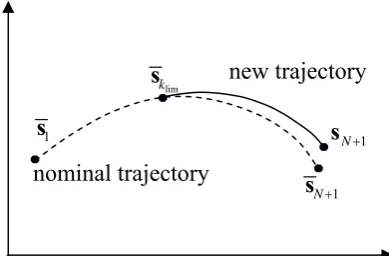
J u s associated to the segment of the trajectory starting at point s_k, if the optimal control policy is employed (see Fig. 1).

Fig. 1 Dynamic programming approach

The value of V_k

 









1 1 1; 1

T

N N N N

V _ s _   s _ t _

dynamic programming requires the solution of Eq. (5) from stage N backward until stage 1. The limitation of dynamic programming for continuous problem is the high dimensional problem resulting from the application of Eq. (5) to every stage k. In fact this is equivalent to find a family of optimal solutions, one from each different initial point s_k,k 1,...,N.

t

1

t t_N1

s

k

u

k

t

k

In order to overcome this computational limitation, differential dynamic programming, applies the principle of optimality in the neighbourhood of a nominal trajectory. At each stage k, the full expression of the stage-wise cost function g and the optimal return function from the next iteration onward V_k1 are replaced by their quadratic approximation about the current nominal control and trajectory.

The state and control vectors at each discretisation step can be written as a variation from their nominal values:

k k k

k k k

 

 

 

s s s

u u u (6)

where the superscript dash indicates the nominal conditions. With this notation,

 

k _k

u is the nominal control profile and

 

k

 

s the corresponding trajectory, obtained by the integration of Eqs. (1) under the nominal control

 

Said QP  the linear and quadratic part of the Taylor expansion of a generic function, differential dynamic programming reduces Eq. (5) to:













k

k k k k k k k k k k k

u

V QP g t V



    _{ }  _ 

 _ _     _

s s  s s u u s s (7)

Similarly to the procedure for solving Eq. (5), the solution of Eq. (7) is performed

backward in time, from the final stage N until the initial stage 1, the boundary condition at t_N1 being:









1 1 1 1 1; 1

T

N N k N k N

V _ s _ s _ QP_  s _ s _ t _ _

The necessary requirement is that the new control sequence should produce small variations in the state vector such that the linear-quadratic approximation in Eq. (7) holds true. This may be achieved even with a big variation in the control action, as long as the time duration of this variation is small. This means that the new control u_k does not need to be restricted to the neighbourhood of u_k, therefore the second of Eqs. (6) can be modified as follows:

*

k  k k

u u u (8)

where the global variation in the nominal control u_k to *

k

 





 

k

k k k k k k k

V _QP g_ t V _{ } __

u

s  s u s (9)

Therefore the linear-quadratic expansion of Eq. (5) is now evaluated about the point

















1 1 1

min , ;

k

k k k _u k k k k k k k k

V QP g t V



     _{ }  _ 

 _{ }     _

s s  s s u u s s (10)

This hypothesis was implemented in an algorithm that employs global variations in the control, hence strong variations in the state (Jacobson and Mayne, 1969; Gerswin and Jacobson, 1970).

The necessary condition to minimise the right hand side of Eq. (10) is to set its first derivative to zero. This leads to the definition of a feedback strategy of the form:

k k k

u  s (11)

The variation in control is expressed as a function proportional to the state variation. Eqs. (9) and (10) are computed backward in time for every stage

,...,1

k N and the coefficient _k is constructed and stored in memory.

At this point, the trajectory is swept forward in time, for every stage k 1,...,N: the successor control policy u_k is constructed and the new trajectory is propagated through the state transition function f , with the initial condition s₁:









* 1 1 1

, ; 1,...,

k k k k k

k k k tk k N

   



 

   

u u s s

s f s u

s s

A posteriori we need to verify that the variations of the control do not break the assumption of linear-quadratic approximations in Eq. (10). To this purpose, a method was proposed by Jacobson and Mayne in 1969 and later refined by Gerswin and Jacobson in 1970, to determine the section of the trajectory over which the new control strategy can be applied.

The nominal control is applied over an initial segment of the trajectory, up to step lim

k , afterwards the new strategy is adopted:

lim *

lim

1,..., 1 ,...,

k k

k k k

k k

k k N



 

  

 



u u

The resulting control law and the associated trajectory are represented respectively in Fig. 2 and Fig. 3:

Fig. 2 Control law schedule according to Jacobson’s algorithm

Fig. 3 Trajectory associated to the control law in Eq. (12)

The guess value of k_lim is initially set to 1 and is progressively increased, until an improvement in the value of the cost function J



 





 



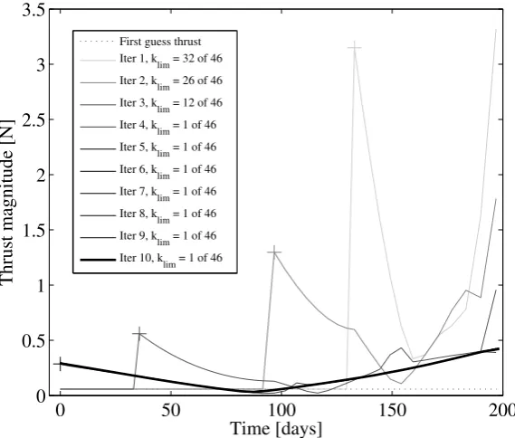
In summary, the core of the DDP technique consists in a backward recursion followed by a forward recursion. A nominal trajectory and control policy are required as input and an improved control law and trajectory are provided as output, which ensures a decrease of the value of the cost function. Successive iterations of the backward and forward recursions produce control laws that progressively approximate the optimal control of the problem. Fig. 4 depicts the history of the control magnitude during the convergence process for a direct transfer from Earth to Mars. The value of k_lim selected at the first iteration of the

1 s

nominal trajectory

new trajectory lim

k

s

1

N

s 1

N

s

k

1 N

u uk

lim

k

algorithm is close to the number of discretisation steps N and tends to 1 as convergence is reached.

0 50 100 150 200

0 0.5 1 1.5 2 2.5 3 3.5

Time [days]

Thrust magnitude [N]

First guess thrust Iter 1, k_lim = 32 of 46

Iter 2, k

lim = 26 of 46

Iter 3, k_lim = 12 of 46

Iter 4, k_lim = 1 of 46

Iter 5, k_lim = 1 of 46

Iter 6, k_lim = 1 of 46

Iter 7, k

lim = 1 of 46

Iter 8, k_lim = 1 of 46

Iter 9, k_lim = 1 of 46

Iter 10, k

lim = 1 of 46

Fig. 4 Control law during the convergence process. Direct transfer Earth to Mars, with a time of

flight of 200 days.

The algorithm has quadratic convergence under the assumption that the Hessian matrix of the cost function is positive definite (Murray, 1978; Murray and Yakowitz, 1984).

The fundamental DDP algorithm

In this section we derive the fundamental DDP algorithm, for an unconstrained problem, starting from the general formulation presented in the previous section. Both sides of Eq. (10) are expanded in Taylor series about the point





,

k k

s u :

 





 

1

1 1 1

1

1 1

1

min , ;

2 1 1 2 2 1 2 k

T k k k

k ss k s k k k k k k k k k s k

k T k T k T k k

u k k ss k k uu k k us k k k s k

T k

k ss k

V V V g t

V V V                             _               _ u

s s s s s u g g s

g u s g s u g u u g s s s

s s



(13)

where _k is defined as the difference between the optimal return function obtained by applying

 

j k

u from the state s_k until the end of the trajectory, and the nominal cost computed by using

 

j k

u from the state s_k until the end of the trajectory:

 

 

k Vk k Vk k

  s  s (14)

Analogously we define k1Vk1

 

 









, ; , ;

k k k k k k k

g g t g t

  s u  s u . The left-hand side of Eq. (13) contains linear and quadratic terms of s_k and the right-hand side contains linear and quadratic terms of s_k, u_k and s_k1, where:









1 1 1 , ; , ;

1 1

2 2

k k k k k k k k k k k

k k T k T k T k

k s k u k k ss k k uu k k us k

t t

  

       

         

     

s s s f s s u u f s u

f f s f u s f s u f u u f s

(15)

with  f_k f s u









1 1 1

min

k

T T T T T

k k k k k k k k k k k k k k k k k

T T

k k k k k k k k k

            _{  }     _               _{ } u

s P s Q s s A s u C u u B s s E

u D g Q f f P f



(16)

1 2 1 k k ss k k s

V n n

V n

 

 

P

Q

denote the linear and quadratic part of the Taylor expansion of the optimal return function at stage k. The matrices A_k, B_k, C_k, D_k and E_k, instead, contains the derivatives of the stage-wise loss function g and the state transition function f at stage k, and the derivatives of the optimal return function of the next stage forward Vk1. If uk and sk are respectively a m1 and n1 vector, we define gu

and g_s to be respectively the 1m and 1n gradient of the scalar cost function g

with respect to the components of the control and the state vector; g_uu, g_ss and

su

g represent the block components of the Hessian matrix of g respectively of size

m m , n n and n m . Said f s u





and with f_uu, f_ss and f_us the blocks components of the Hessian matrix of f respectively of size m m n  , n n n  and n m n  . All the above quantities are evaluated at





1 1 1

1

1 1 1

1

1 1 1

1 1 2 1 2 n

k k k k T k k k k

k ss s j ss j s ss s k ss ss

j

T n

k k k k T k k k k

k su s j su j s ss u k ss su

j n

k k k k T k k k

k uu s j uu j u ss u k ss

j

V V V n n

V V V m n

V V V

             _{   }   _  _{   }    _     _{   }  _  _{   }    _          _{   }   







A g f f f f f

B g f f f f f

C g f f f f f









k k k T k k

k u s u k ss u

T

k k k T k k

k s s s k ss s

m m

V V m

V V n

      _              

D g f f f

E g f f f

(17)

Note that the last terms of the matrices A_k, B_k and C_k have to be rewritten in order to represent a quadratic form respectively with respect to













1 1 1

T

k k k k k k k k

     g Q   f f P f (18)

1 0

N

  (19)

The value of u*_k in Eq. (8) is computed by solving the minimisation problem on the right hand side of Eq. (9), which is equivalent to solving the right hand side of of Eq. (16) for s_k and u_kset to zero:

* 1 1

min

k

T

k k k k k k

      

 

u g Q f f P f

(20)

As a consequence at *

k

u the following condition is satisfied:

1 1 1 1 1

0 0 0

2

k T k k k k T k k

u k Vs k kVss k u Vs u kVss u k

   

 

  _     _       

 g f f f  g f f f D

Once *

k

u is computed, problem Eq. (16) can be solved with respect to u_k. The necessary condition for the minimisation of Eq. (16) with respect to u_k implies that:

1 1

2 0

2

k k k k  k k k k



    

C u B s u C B s (21)

Eq. (21) gives the coefficient _k of the feedback control law in Eq. (11):

1 1 2

k k k m n



  C B  (22)

The variation in control in Eq. (21) can be substituted back in Eq. (16) and by grouping the terms of the same order we obtain:

1 1 4 T k k T

k k k k k





 

Q E

P A B C B (23)

with the final conditions:









1 1 1

1 1 1

; 1

; 2

T

N N N _s

T

N N N _ss

t t           _  _    _  _ Q s P s (24)

Eqs. (20), (17), (18), (22) and (23) are computed backward in time for every stage ,...,1

k N with the final condition Eqs. (19) and (24) at stage N+1 and the coefficient

 

DDP ensures an improvement at each iteration under the condition that the Hessian of the cost function, i.e., the matrix C_k is positive definite. In case this is not verified, different procedures can be applied (see Mayne, 1966; Jacobson and Mayne, 1969; Yakowitz and Rutherford, 1984; Liao and Shoemaker, 1992). The one implemented in this work replaces the matrix C_k, for the computation of Eq. (22), with the positive definite matrix

 

min 2

k  k   m

C C (25)

where _min is the minimum eigenvalue of the matrix C_k and  m the identity matrix of size m.

The condition on the matrix C_k is even more stringent; in fact, in order to achieve a sufficient descend direction at each iteration, the matrix C_k should also be far from non-positive definite condition (Gill et al., 1981); hence the active shift Eq. (25) is applied, also in case the minimum eigenvalue _min, although positive, is smaller than a given small positive value (10-6 was usually adopted).

Once the backward propagation is terminated, the trajectory is swept forward in time, for every stage k1,...,N ; the new control policy is given by Eq. (12) and the corresponding trajectory is computed by Eq. (1). The value of k_lim in Eq. (12) has to be chosen such that the following condition is satisfied, c being a constant between 0 and 1.

 







 



J u s J u s  c (26)

where J



 



lim

k

 is used as a measure of the predicted change in cost applying the control law Eq. (12). A single iteration of DDP is composed by the backward and the forward recursion that produce an improved control law and trajectory. A number of iterations follow one after the other, until the stopping condition

1 out

   (27)

Treatment of the terminal equality constraints

The terminal constraints are added to the cost function through a set of Lagrange multipliers to give the Lagrange function in Eq. (4).

In this paper we follow the method proposed by Gershwin and Jacobson (1970). At first Eq. (4) is minimised fixing the value of the Lagrange multipliers . Successive iterations of DDP follow until the convergence criterion Eq. (27) is satisfied. At this point a variation of  is allowed, in order to find a control law that decreases the constraints violation. Eq. (5) is now expanded not only in u_k and s_k but also in  about the point





 





 

1 1 1

1 1 1 1 1

1 1 1 2 2 1 1 , ; 2 2 1 2 1 2

T k T k T k k k

k ss k k s s k k k k

k k T k T k

k k k k k s k u k k ss k k uu k

T k k T k k

k us k k k s k k ss k

T k

k

V V V V V V

g t

V V V V

V                                                                 

s s s s s

s u g g s g u s g s u g u

u g s s s s s

s 1 1

T k

s V_

(28)

Substituting Eq. (15) and grouping some terms, Eq. (28) can be written in a matrix form:

1 1 1

T T T

k k k k k k k k k k

T T T T T

k k k k k k k k k k k k k

T T T

k k k k k k k

                 _     _ _                   

s P s R s S Q s Z

s A s u C u u B s s E u D

R s H u K Z

(29)

where some more matrices are introduced for clarity; respectively on the left side:

 

V l l

V n l

         Z R S (30)













k T k k T

k s s s k

k T k k T

k u s u k

k k

V l l

V n l

V m l

V l                       R

H f f S

K f f S

Z

(31)

Note that the variation of Lagrange multipliers is introduced only once an optimal control law has been found with  ; as a consequence, from Eq. (28), u*_k u_k and hence  g_k 0 and  f_k 0 . This is equivalent to use the small control variation algorithm (Jacobson and Mayne, 1979). Now, by differentiating Eq. (29) with respect to u_k we obtain:

1 1

2 0

1 1

2 2

k k k k k

k k k k k k

  

    

   

  

C u B s K

u C B s C K

Hence the variation of the control contains also a term proportional to the variation of the multipliers:

k k k k

u  s   (32)

The associated coefficient _k is computed during the backward recursion and stored in memory together with coefficient _k:

1 1 2

k k k m l



  C K  (33)

By substituting back Eq. (32) in Eq. (29) we obtain: 1 1 1 1 1 2 1 4 T

k k k k k

T

k k k k k

k k         

S H B C K

R R K C K

Z Z

(34)

with the final conditions:









1 1 1

1

1 1 1

;

;

T

N s N N

N

N N N

The backward recursion is performed for every stage k N,...,1, in which the same equations of the main DDP loop are solved, with the addition of Eqs. (31), (33) and (34), with the final condition Eqs. (35); the coefficients

 

 

N

k _k are stored in memory.

At this point we can determine the variation of Lagrange multipliers  , by maximising Eq. (28) at t₁ and s₁, with respect to  (see Jacobson and Mayne, 1969); this gives:

1 1 1 2

T

   R Z (36)

under the requirement that R₁ is negative definite (hence invertible).

The new control law and trajectory are propagated for every stage k 1,...,N:





1 1 1

, ; 1,...,

k k k k k

k k k tk k N

 



  



 _{ }

   

u u s

s f s u

s s

(37)

Also in this case,  has to be verified not to exceed the range of validity of the linear-quadratic expansion, hence the constant 0  1 is introduced in Eq. (36):

1 1 1

0 1

2

T

  



   

 

R Z

(38)

The value of  is chosen, through a linear search method, so that the following condition is satisfied (Gershwin and Jacobson, 1970):

 







 













 



1 1 1

2 1

1 1 1 1 1 1

, ; , ;

1 1

; ; ;

2 2

k k

T

N N N N k

J J

t t reltol J



   

   

   

 

 _  _ 

 

u s u s

s R s u s

(39)

where reltol is a relative tolerance. Eq. (39) compares the actual improvement in the cost function to the one predicted through the linear-quadratic expansion. Moreover the change in has to reduce the violation of the terminal constraints:



 



3 Modified

DDP

method

When the optimisation problem is not very sensitive, for example when designing a two-body problem transfer, the conventional DDP technique, described in paragraph 2, can be applied to find the optimal control. However if the problem involves a more complex dynamics, such as escape or capture phases, or gravity assist passages, the propagation of the dynamics becomes a crucial point. In particular, the use of a time mesh fixed a priori can jeopardise the high fidelity representation of the problem; on the other hand, the coupling between the integration scheme and the optimisation process must be handled very carefully, in order not to compromise convergence.

The approach proposed in this paper uses a variable step integration method for the propagation of the dynamics and the integration mesh is refined at each iteration of DDP.

3.1 Discretisation scheme

The low-thrust continuous problem, characterised by the dynamic system:

 





 

0 0 1

, ; _f

t t t t t t t

t

  _ _



s f s u

s s

 

(41)

is approximated by difference equations as shown in Eq. (1), where the state transition function f represents the explicit scheme for the numerical approximation of Eq. (41):









1 1 1

, , ; ; 1,...,

k  k k k tk hk k N



s f s f s u

s s



(42)

where h_k is the discretisation step. Note that in the rest of the paper the dependences of the function f were written in the simplified form:













f s u f s f s u

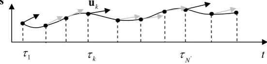
Fig. 5 Trajectory discretisation within the optimisation problem.

In a previous application of the discrete-time DDP algorithm to orbital transfer, a fixed step size Euler integration scheme was used (see Gershwin and Jacobson, 1970). However, such a simple integration scheme is not appropriate when the dynamics becomes highly non-linear. In other more recent DDP-based approaches, the issue was solved by dividing the trajectory in a number of segments over which the thrust is constant (Whiffen, 2002; Lantoine and Russell, 2008). Within a single segment Whiffen integrates backward a system of coupled ordinary differential equations which are the integral form of the discrete-time DDP matrices, while Lantoine and Russel introduce a second order state transition matrix to map the propagation of the dynamics. In these approaches, decision times and integration steps do not coincide.

In our work, the classical discrete formulation is used (see Fig. 5) but the mesh is discretised with a scheme more accurate than the one adopted by Gershwin and Jacobson (1970): a variable step-size Runge-Kutta-Fehlberg integration scheme, with a six stage pair of approximation of the forth and fifth order (Dormand and Prince, 1980):





1

1 ,

1 , ;

, ; 1,..., ; 6

k k k k k k r r

r

r k k j r r k k r k

r

t h

h t h j

 

 







  

 

 _   _  

 





s f s u s b f

f f s a f u c



  

(43)

where f is the continuous dynamic of the problem, a, b and c the coefficient matrices of the integration scheme and h_k the length of the discretisation step. Note that the integration scheme Eq. (43) was chosen to be explicit, as it allows the analytic evaluation of its derivatives which are required in the DDP procedure (in Eqs. (17) and Eqs. (31)).

t

1

t _tN1

s uk

k

The identity between decision times and integration steps increases the computational requirements but ensures high fidelity of the dynamics and allows varying the control at each integration step.

Note that, if u_k is kept constant over a certain number of discretisation steps, Eq. (43) reduces to the trajectory model used by Whiffen and Lantoine (see Fig. 6).

Fig. 6 Trajectory discretisation in the Static/Dynamic Control approach. The gray arrows show that

the control is kept constant within a segment.

3.2 Mesh definition

If the dynamic system Eq. (42) is not correctly integrated, the optimisation of the control law could lead to an incorrect solution. This is likely to occur if a fixed step size is used.

For this reason, in the approach proposed in this paper, the step-size of the integration scheme was adapted at each iteration of the DDP algorithm.

We define a nominal time-mesh grid

 

 

 

Once a value of k_lim is determined, according to condition Eq. (26), the trajectory selected for the next DDP iteration follows, within the range





 

lim 1

N k k k

 

s implements the new control strategy

 

lim

N k k k

u , according to Eq. (12). The segment

 

lim 1

N k k k

 

s of the trajectory is propagated through the adaptive-step integration algorithm and a new mesh

 

 

lim 1

N k k k

 

s and

 

N k k k

u .

In order to perform this operation, the control law, which is given on the original mesh points, needs to be interpolated in the new points required by the integration algorithm. Handling properly the interpolation is essential to preserve the DDP

t

1

 _'

N



s

k



k

performances; in fact a bad interpolation could introduce errors which can results in rejecting the control computed by the DDP.

Two interpolation schemes were adopted in this study; the first one, called

complete interpolation in the following, directly interpolates the control

 

N k k k u

on the new mesh. Recalling Eq. (12), the complete interpolation technique interpolates the left hand side of Eq. (44):





*

lim,...,

k  k  k k k kk N

u u s s (44)

The second interpolation technique, although more computationally expensive, ensures a higher accuracy. Rather than interpolating the control computed on the nominal mesh through the forward recursion

 

lim

N k _{k k}

u , each term on the right hand side of Eq. (44), namely *

k

u , _k s_k, is independently interpolated. In this way the feedback nature of the control variation computed by the DDP is fully exploited: if the state

 

lim 1

N k _{k k}

 

s moves away from the one computed on the nominal mesh

 

lim 1

N k _{k k}

 

s , the term of the control _k





In some cases (see the transfer problem presented in section 5.1) the complete interpolation technique is enough to reach convergence, while in more sensitive and complex cases, the complete interpolation introduces small errors in the interpolated control that, propagated through a sensitive dynamics, may result in an unrecoverable increase of the final constraints violation. For example for the transfer problem presented in section 5.2, the tem-wise interpolation technique was essential to reach the convergence. In particular, the section of the trajectory where the spacecraft passes close to the Earth gravity field, highlighted in Fig. 18, showed to be very sensitive to the control profile and hence required a very high accuracy in the control law interpolation.

 







 





 



N N N

k _k k _k mesh k _k mesh

J u _ s J u _ s reltol J u _ s reltol  (45) By using the term-wise interpolation technique, condition Eq. (45) was always satisfied. In the cases in which the complete interpolation technique was adopted, instead, Eq. (45) was used as verification of the failure of the interpolation technique; when that occurred, the DDP mesh refinement was performed again, with the term-wise interpolation technique.

Note that the mesh refinement during the optimisation process increases the computational time, but only in this way one can ensure that the algorithm convergences to a correct solution.

4 Algorithm

We now report a summary of the algorithm adopted in this work. The algorithm is composed by the following steps:

Initialisation

A nominal set of Lagrange multipliers and a control law

 

 

 



 



associated to the nominal strategy and trajectory is evaluated through Eq. (4). Moreover the derivatives of the state transition function and the stage-wise loss function g are analytically computed.

Loop1: Control law loop

Step 1: The parameters needed for starting the recursive computation of Eq. (16) are initialised at step N1, through Eq. (19) and Eqs. (24), computed with the nominal value of the Lagrange multipliers .

Step 2: Backward propagation performed for each stage k from stage N to backward until stage 1:

subspace trust-region method, based on the interior-reflective Newton method (Coleman and Li, 1996; Coleman and Li, 1994). The analytic expression of the gradient is supplied.

The derivative of the state transition function and the stage-wise loss function g

are evaluated at





Eq. (18) represents the prevision of the improvement in the cost function associated with stage k, while the matrices Q_k and P_k are computed through Eq. (23) and replaced to the one of the next step forward. The coefficient _k is computed with Eq. (22) and stored in memory for the forward propagation. If the matrix C_k is not positive definite, Eq. (25) is used for the computation of _k:

1 1 2

k k k m n



  C B 

Step 3: Forward propagation performed from step 1 to step N.

The trajectory is propagated through Eq. (1), with the improved control law Eq. (12). The value of k_lim is determined through Eq. (26), to provide a decrease in the objective function, and not to exceed the range of accuracy of the linear-quadratic expansion. The constant c in Eq. (26) was set in a value between 0.5 and 0.1.

Step 4: When a new control sequence

 

N k _k

u is selected, the corresponding leg of trajectory is integrated with the adaptive step integration method, by interpolating the control through the complete interpolation technique or the term-wise interpolation technique, and a new discretisation of the control is obtained

 

N k k

u . The value of the cost function associated to the new discretisation and the value computed on the original mesh are compared through Eq. (45).

The new mesh, together with the improved control law and the associated trajectory are set as the nominal conditions for the next DDP iteration (Step 1).

 

 

 

 

 

 

 







 



1 1

1 1

1 1

1 1

1; 1;

N N

k k k k

N N

k k k k

N N

k k k k

N N

J J

 

 

 

 

   

u u

s s

Convergence Criterion:

The first loop of DDP is stopped when k_lim 1 and the increase of the cost function is under a small value, set for stability analysis:

 





1 max 1, 1; 1

N

out  J k _k 

    _{ }

 u s  (46)

Usually _out is set to be around 10-6 but it can be increased up to 10-4 if the problem is very sensitive in order to filter the numerical error introduced by the integration over a long time of flight.

Loop 2: Equality constraints loop

Step 5: Backward propagation performed for each stage k from stage N to backward until stage 1:

The matrices in Eq. (17) and Eq. (23) are constructed, together with the new matrices in Eq. (31) and Eq. (34) with the initial condition Eqs. (24) and Eq. (35). All the derivatives are now evaluated at point





Coefficients _k and _k are computed through Eq. (22) and Eq. (33) and stored in memory for the forward propagation.

Step 6: Forward propagation performed from step 1 to step N.

The value of the Lagrange multiplier vector is updated with Eq. (38) and the new control law is propagated with Eq. (37). The value of  is set according to condition Eq. (39).

Test on the final constraints:

The violation of the constraints is updated and, if condition Eq. (40) is verified, the new value of is set as the nominal one, together with the control sequence and trajectory; else  is further decreased. The algorithm goes back to Step 1 for further DDP iteration.

Stopping condition

The overall algorithm terminates at the end of loop 1, if condition Eq. (46) is satisfied and the constraints violation is under a required tolerance.

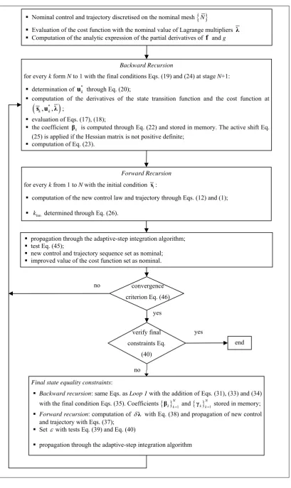
Fig. 7 Modified DDP algorithm.

Final state equality constraints:

 Backward recursion: same Eqs. as Loop 1 with the addition of Eqs. (31), (33) and (34)

with the final condition Eqs. (35). Coefficients  k kN₁ and   1

N

k k stored in memory;

 Forward recursion: computation of  with Eq. (38) and propagation of new control

and trajectory with Eqs. (37);

 Set  with tests Eq. (39) and Eq. (40)

 propagation through the adaptive-step integration algorithm

 Nominal control and trajectory discretised on the nominal mesh

 

 Evaluation of the cost function with the nominal value of Lagrange multipliers

 Computation of the analytic expression of the partial derivatives of f and g

Backward Recursion

for every k form N to 1 with the final conditions Eqs. (19) and (24) at stage N+1:

 determination of u*_k through Eq. (20);

 computation of the derivatives of the state transition function and the cost function at





, ,

k k

s u ;

 evaluation of Eqs. (17), (18);

 the coefficient k is computed through Eq. (22) and stored in memory. The active shift Eq.

(25) is applied if the Hessian matrix is not positive definite;

 computation of Eq. (23).

Forward Recursion

for every k from 1 to N with the initial condition s1:

 computation of the new control law and trajectory through Eqs. (12) and (1);

 klim determined through Eq. (26).

convergence criterion Eq. (46)

verify final constraints Eq.

(40)

end yes

yes

no no

 propagation through the adaptive-step integration algorithm;

 test Eq. (45);

 new control and trajectory sequence set as nominal;