Dynamic Programming and Mean-Variance Hedging in Discrete Time

City, University of London Institutional Repository

Citation

:

10.1080/1350486042000196164

This is the accepted version of the paper.

This version of the publication may differ from the final published

version.

Permanent repository link:

Link to published version

:

Copyright and reuse:

City Research Online aims to make research

outputs of City, University of London available to a wider audience.

Copyright and Moral Rights remain with the author(s) and/or copyright

holders. URLs from City Research Online may be freely distributed and

linked to.

City Research Online: http://openaccess.city.ac.uk/ publications@city.ac.uk

Dynamic Programming and Mean-Variance Hedging in

Discrete Time

AlešCerný (ˇ a.cerny@imperial.ac.uk)

The Business School, Imperial College London Forthcoming in Applied Mathematical Finance

First draft: April 1999, this version October 2003

typo in Theorem 3 (time subscripts in expression forεt) corrected 15/10/2004

Abstract. In this paper we solve the general discrete time mean-variance hedging problem by dynamic programming. Thanks to its simple recursive structure our solution is well suited for computer implementation. On the theoretical side, we show how the variance-optimal measure arises in our dynamic programming solution and how one can define conditional expectations under this (generally non-equivalent) measure. We are then able to relate our result to the results of previous studies in continuous time, namely Rheinländer and Schweizer (1997), Gourieroux et al. (1998), and Laurent and Pham (1999).

Keywords: mean-variance hedging, discrete time, dynamic programming, incom-plete market, arbitrage

JEL classification code:G11, C61

Mathematics subject classification:90A09, 90C39

1. Introduction

This paper gives a dynamic programming solution to the general dis-crete time mean-variance hedging problem, a solution which from the practical point of view is well suited for computer implementation thanks to its recursive structure. We show how the optimal strat-egy hedging is implemented on a spreadsheet for the case with lep-tokurtic IID stock returns. On the theoretical side, we show how the variance-optimal measure arises in the dynamic programming solution and how one defines conditional expectations under this (generally non-equivalent) measure. We are then able to relate our result to the results of previous studies in continuous time.

The mean-variance hedging in continuous time has been tackled via Galtchouk-Kunita-Watanabe decomposition under a suitable, so-called variance-optimal, martingale measure. The problem was first formulated in Duffie and Richardson (1991), Schweizer (1992) obtained

∗ _{I wish to thank Martin Schweizer and three anonymous referees for valuable}

the first ground breaking result under the assumption of a so-called

constant investment opportunity set.This special case has the property that the variance-optimal measure coincides with the so-called minimal martingale measure of Föllmer and Schweizer (1991). A fully general

solution was finally obtained by Rheinländer and Schweizer (1997)

and Gourieroux et al. (1998), the latter using an elegant numeraire method. Laurent and Pham (1999) used the framework of Gourieroux et al. (1998) coupled with duality theory and dynamic programming to calculate explicit characterization of the variance-optimal measure in stochastic volatility models.

Studies of mean-variance hedging in discrete time are relatively few. Schäl (1994) applies dynamic programming in the case of constant investment opportunity set to examine various intertemporal mean-variance criteria. Schweizer (1995) solves the general problem with one asset and non-stochastic interest rate. This solution, however, does not have fully recursive structure. Namely, it requires calculation of two processes(β_t)t=0,1,...,T−1and(ρt)t=0,1,...,T−1as conditional expectations

of T-measurable variables at every node of the state space, which is computationally inefficient — in a recombining trinomial tree it requires in the order of 3T−t operations at every node at time t and for all t. In the same situation, a fully recursive dynamic programming solution requires only3operations at every node and at all times. Such solution has been derived, independently of our work, by Bertsimas et al. (2001) for one basis asset and non-stochastic interest rate1.

The present paper can be seen as an extension of Schäl (1994) to the case of non-constant investment opportunity set and several risky assets. The contribution of our paper is threefold. Firstly, unlike Schweizer (1995) and Bertsimas et al. (2001) we solve the hedging problem with stochastic interest rate (and an arbitrary number of basis assets). Secondly, we give a simple recursive solution which in Markov setting improves greatly on the computational efficiency compared to the result of Schweizer (1995). Last but not least, by suitably defining the conditional expectation under the non-equivalent variance-optimal measure we are able to link our discrete time results to the continuous-time results of Rheinländer and Schweizer (1997), Gourieroux, Laurent, and Pham (1998), and Laurent and Pham (1999).

1

Bertsimas et al. (2001) solve the hedging problem with rt = 0,claiming that this entails no loss of generality. What they mean is that with stochastic interest rate they are able to minimizeE0

h¡

V_Tx,θ₋HT¢2/¡ST0

¢2i

. Of course, the economically interesting problem is that of minimizing E0

h¡

The paper is organized as follows: In thefirst section we present the main result. The second section gives an explicit example with fat-tailed return distribution and weekly rebalancing period. In the third sec-tion we show how the variance-optimal measure arises in the dynamic programming solution, how one defines conditional expectations under this measure and how the existence of the variance-optimal measure is related to the no-arbitrage assumption. Thefinal section relates our result to the results of previous studies in discrete and continuous time.

1.1. Notation

Let us have a filtered probability space (Ω,_F,_P,_{Ft}t∈T) with EPt

denoting the expectation conditional on the information at timet

EP_t [X] _≡ EP[X_|Ft],

T = _{0,1, . . . , T_}.

To keep the technicalities at minimum we will assume thatΩisfinite2, that is the information structure can be represented by a tree. The conditional expectation EP_t [X]assigns one value to each node at time t in the information tree.

All processes defined in the next section, except for the cumulative discountS0,are adapted. For a process_{Xt}t∈T being adapted means

that the value ofXt is known at timet but that generally the value of

Xt is uncertain as oft−1.The processS0 is predictable, that isSt0 is

known already at time t₋1.

Measurability is important for manipulation of conditional expecta-tions, for example we will frequently use the fact that

EP_t [XtY] =XtEPt [Y],

and vice versa. The only other tool we need is the law of iterated expectations

EP_t hEP_s [X]i= EP_t [X],

whenever s_≥t.Matrix transpose is denoted by asterisk∗.

2. Mean-square hedging in discrete time

Suppose that there are n basis assets with _Rn-valued price process S = (St)t=0,...,T and dividend process δ = (δt)t=1,...,T. Assume further

that there is a risk-free short term borrowing and lending with return Rft and define the cumulative discount

S_t0 = Rf0×Rf1×. . .×Rft−1,

S₀0 = 1.

Let us define the discounted gain process of the basis assets X

Xt ≡

St

S_t0 +

t X

i=1

δi

S_i0,

∆Xt ≡ Xt−Xt−1.

Process Vx,θ denotes the wealth obtained by self-financing strategy with initial investment x and with shares of risky investment given by the portfolio process θ= (θt)t=0,...,T−1.

V_tx,θ = Rft−1Vtx,−1θ+St0θ∗t−1∆Xt (1)

∆

Ã

Vx,θ S0

!

t−1

= θ∗_t−1∆Xt (2)

V_tx,θ

S_t0 = x+

t−1 X

i=0

θ∗_i∆Xi+1.

In what follows it is important to capture the fact that some processes are unaffected by the choice of the trading strategy.

DEFINITION 1. A random variableX :Ω_→Ris called exogenous if

for every fixed ω_∈Ω the value X(ω) does not depend on the choice of

V₀x,θ(ω),θ0(ω), . . . ,θT−1(ω).

We assume that processes X and S0 _{are exogenous; this is a}

stan-dard assumption in finance literature, its relaxation has been studied prominently by Frey and Stremme (1997); see alsoCerný (1999). Givenˇ

an exogenous and _FT-measurable payoff HT the best mean-square

hedge for HT is given by the initial wealth x and portfolio weights

θ which are found by minimizing the expected square replication error

EP₀ hV_Tx,θ₋HT i2

min

x,θ0,...,θT−1 EP₀

 

Ã

S_T0

Ã

x+

T_X−1

i=0

θ∗_i∆Xi+1 !

−HT

!2



THEOREM 2 (Optimal controls). LetktandHtbeFt-measurable and

exogenous, with kt > 0 a.s. Assume further that there is no arbitrage

among the basis assets, which in particular implies Rft−1 >0, and that

the excess returns of basis assets are linearly independent.

Then the matrix EP

t−1[kt∆Xt∆Xt∗] is invertible at each node of the

information set _Ft−1 and the problem

min

x,θ0,...,θt−1 EP₀

·

kt ³

V_tx,θ₋Ht ´2¸

(3)

has the same optimal controls x,θ0, . . . ,θt−2 as the problem

min

x,θ0,...,θt−2 EP₀

·

kt−1 ³

V_tx,₋θ₁₋Ht−1 ´2¸

(4)

with kt−1 >0 and Ht−1 beingFt−1-measurable and exogenous

kt−1

R2 ft−1

= EP_t−1[kt]−EPt−1[kt∆Xt∗] ³

EP_t−1[kt∆Xt∆Xt∗] ´−1

EP_t−1[kt∆Xt],

(5)

Ht−1 = EP_t−1

·µ

kt−EPt−1[kt∆Xt∗] ³

EP_t−1[kt∆Xt∆Xt∗] ´−1

kt∆Xt ¶

Ht

Rft−1

¸

kt−1

R2

ft−1

,

(6)

and the dynamically optimal value of θt−1 is given as

θD_t−1 =₋³EP_t−1[kt∆Xt∆Xt∗] ´−1

EP_t−1  kt∆Xt

 V

x,ˆθ t−1

S_t0₋₁ − Ht

S_t0

   . (7)

Proof. See Appendix A.

THEOREM 3 (Value function). Let kT >0andHT beFT-measurable

random variables. Then

min θt,...,θT−1

EP_t

·

kT ³

V_Tx,θ₋HT ´2¸

=kt ³

V_tx,θ₋Ht ´2

+ε2_t

where _{ε_} is a well-defined _F-adapted exogenous process satisfying

ε2_t = EP_t hε2_t+1i+ EP_t

·

kt+1 ³

RftHt+St0+1 ³

¯

θD_t ´∗∆Xt+1−Ht+1 ´2¸

,

ε2_T = 0,

where ¯θD_t−1 is obtained from (7) by substituting Ht−1 for Vx,θ

D

t−1 ,that is,

¯_θD t−1 =−

³

EP_t−1[kt∆Xt∆Xt∗] ´−1

EP_t−1

"

kt∆Xt Ã

Ht−1

S0 t−1

−H_S0t t

!#

Proof. See Appendix A.

COROLLARY 4. Theorems 2 and 3 provide complete characterization

of the solution to the mean-variance hedging problem. A repeated appli-cation of the theorems starting from T withkT = 1 gives us all values

of kt and Ht for 0 ≤ t ≤ T. Further, at the end of the backward run

we learn that the optimal value of initial wealth is xˆ=H0 and that the

expected squared hedging error is ε2₀.In a forward run from time 0 we can then recover the optimal portfolio and optimal hedging wealth from (7) and (1). If Xt is Markov, the interest rate is non-stochastic and

HT is a European contingent claim,HT =H(XT),then it follows from

(5) and (6) that the processes kt, Ht, ¯θDt−1 and ε2t depend only on one

state variable, Xt. The optimal wealth VH0,θ

D

t , however, is - save for

very special cases - path dependent, see Schweizer (1998).

3. Discrete Time Hedging with IID Returns

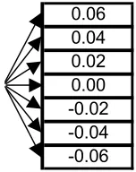
In this section we illustrate how the dynamic programming solution can be usefully applied in practice. We will consider trading once a week for 6 weeks. We assume that weekly log-returns are spaced regularly with 2% gap, see Figure 1.

0.06 0.04 0.02 0.00 -0.02 -0.04 -0.06

Figure 1. Logarithm of weekly stock returns.

The conditional objective probabilities of movement in the lattice are calibrated from historical data, based on the FTSE 100 weekly returns in the period 1984-2001, see Figure 2.

0.013 0.067 0.273 0.384 0.199 0.050 0.014

Figure 2. Conditional objective probabilities of stock price movement.

larger number of state variables. Such extensions, however, are beyond the scope of this illustrative section.

Our aim is to hedge a European call option with 6 weeks to expiry, rehedging once a week. We will assume that the initial value of the index isS0 = 100and that the option is struck at the money K= 100.

The resulting stock price lattice is depicted in Figure 3.

3.1. Mean value process H

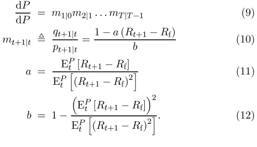
This process could be computed directly from equation (6), but in an IID model it is most conveniently constructed with the help of special risk-neutral probabilities called variance-optimal probabilities, see equation (18). The variance-optimal probabilities in turn are com-puted from the distribution of excess return. The variance-optimal measure will be denoted P˜ to distinguish it from the objective proba-bility measure P. The corresponding change of measure is given by the formula

d ˜P

dP = m1|0m2|1. . . mT|T−1 (9)

m_t+1|t , qt+1|t p_t+1|t =

1₋a(Rt+1−Rf)

b (10)

a = E

P

t [Rt+1−Rf] EP

t h

(Rt+1−Rf)2

i (11)

b = 1₋

³

EP_t [Rt+1−Rf]

´2

EP t

h

(Rt+1−Rf)2

t=6

143.33 t=5 140.49 137.71 134.99 134.99 t=4 132.31 132.31 129.69 129.69 127.12 127.12 127.12 t=3 124.61 124.61 124.61 122.14 122.14 122.14 119.72 119.72 119.72 119.72 t=2 117.35 117.35 117.35 117.35 115.03 115.03 115.03 115.03 112.75 112.75 112.75 112.75 112.75 t=1 110.52 110.52 110.52 110.52 110.52 108.33 108.33 108.33 108.33 108.33 106.18 106.18 106.18 106.18 106.18 106.18 t=0 104.08 104.08 104.08 104.08 104.08 104.08 102.02 102.02 102.02 102.02 102.02 102.02 100.00 100.00 100.00 100.00 100.00 100.00 100.00 98.02 98.02 98.02 98.02 98.02 98.02 96.08 96.08 96.08 96.08 96.08 96.08 94.18 94.18 94.18 94.18 94.18 94.18 92.31 92.31 92.31 92.31 92.31 90.48 90.48 90.48 90.48 90.48 88.69 88.69 88.69 88.69 88.69 86.94 86.94 86.94 86.94 85.21 85.21 85.21 85.21 83.53 83.53 83.53 83.53 81.87 81.87 81.87 80.25 80.25 80.25 78.66 78.66 78.66 77.11 77.11 75.58 75.58 74.08 74.08 72.61 71.18 69.77

Figure 3. Stock price lattice.

Numerically,

Rt+1 =£e0.06 e0.04 e0.02 e0.00 e−0.02 e−0.04 e−0.06¤,

Rf= 1.00075, Rt+1−Rf

=£6.108 4.006 1.945 ₋0.075 ₋2.056 ₋3.997 ₋5.899¤_×10−2,

EP_t [Rt+1−Rf] = 1.58×10−3, EPt h

(Rt+1−Rf)2

i

a= 1.58×10− 3

4.72_×10−4 = 3.35

b= 1₋1.58 2

×10−6

4.72_×10−4 = 0.9947

m_t+1|t=£0.7995 0.8704 0.9398 1.007 9 1.0746 1.1400 1.2041¤

q_t+1|t=m_t+1|tp_t+1|t

=£0.010 0.058 0.257 0.387 0.214 0.057 0.017¤

The risk-neutral probabilitiesq and the option payoffHT define the

mean value process_{Ht}t=0,1,...,T as follows

Ht= E ˜ P t

"

HT

RT_f−t

#

In our special case with IID returns and deterministic interest rate the conditional variance-optimal probabilities q_t+1|t coincide with the risk-neutral probabilities of one-period Markowitz CAPM model. Thus HT−1 is the CAPM price of the option at time T −1, HT−2 is the

CAPM price of HT−1 at timeT −2 and so on.

The value ofHtis computed recursively using the risk-neutral

prob-abilities and starting from the last period as in the complete market case

Ht = E

˜ P t

·_H

t+1

Rf

¸

, (13)

t = T₋1, . . . ,0.

However, formula (13) differs from its complete market counterpart in one important aspect. While in a complete market there is a

self-financing portfolio with value Ht that perfectly replicates Ht+1, in an

incomplete market such a portfolio generally does not exist.

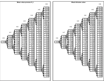
The mean value processHtis depicted in Figure 4, together with

cor-responding continuous Black—Scholes value for comparison. Consider,

for example the middle node at t = 1. The Black—Scholes formula

dictates

C(S, K, r,σ,τ) =SΦ

Ã

ln_KS + (r+ σ₂2)τ σ√τ

!

−e−rτKΦ

Ã

ln_KS + (r₋σ₂2)τ σ√τ

!

with

S = 100, K= 100, r = lnRf= 7.5×10−4,

σ =

q

VarP_t (lnRt+1) = 2.165×10−2,

resulting in C= 2.12 as compared to H= 2.09.

t=6 t=6

43.33 43.33

t=5 40.49 t=5 40.49

37.71 37.71

35.06 34.99 35.06 34.99

t=4 32.39 32.31 t=4 32.39 32.31

29.77 29.69 29.77 29.69

27.28 27.20 27.12 27.28 27.20 27.12

t=3 24.76 24.68 24.61 t=3 24.76 24.68 24.61

22.29 22.22 22.14 22.29 22.22 22.14

19.95 19.87 19.80 19.72 19.95 19.87 19.80 19.72

t=2 17.58 17.50 17.43 17.35 t=2 17.58 17.50 17.43 17.35

15.25 15.18 15.10 15.03 15.25 15.18 15.10 15.03

13.06 12.98 12.90 12.83 12.75 13.05 12.98 12.90 12.83 12.75

t=1 10.83 10.75 10.67 10.59 10.52 t=1 10.83 10.75 10.67 10.59 10.52

8.68 8.58 8.48 8.40 8.33 8.68 8.57 8.48 8.40 8.33

6.78 6.63 6.49 6.36 6.26 6.18 6.78 6.63 6.49 6.36 6.26 6.18

t=0 4.95 4.75 4.56 4.36 4.19 4.08 t=0 4.95 4.76 4.56 4.36 4.18 4.08

3.36 3.13 2.87 2.59 2.27 2.02 3.38 3.14 2.89 2.61 2.29 2.02

2.32 2.09 1.85 1.57 1.24 0.82 0.00 2.35 2.12 1.88 1.61 1.30 0.90 0.00

1.18 0.96 0.72 0.45 0.16 0.00 1.21 1.00 0.77 0.51 0.22 0.00

0.59 0.43 0.27 0.12 0.02 0.00 0.62 0.46 0.30 0.15 0.03 0.00

0.26 0.16 0.08 0.02 0.00 0.00 0.29 0.19 0.10 0.03 0.00 0.00

0.05 0.02 0.00 0.00 0.00 0.06 0.03 0.00 0.00 0.00

0.01 0.00 0.00 0.00 0.00 0.02 0.01 0.00 0.00 0.00

0.00 0.00 0.00 0.00 0.00 0.00 0.00 0.00 0.00 0.00

0.00 0.00 0.00 0.00 0.00 0.00 0.00 0.00

0.00 0.00 0.00 0.00 0.00 0.00 0.00 0.00

0.00 0.00 0.00 0.00 0.00 0.00 0.00 0.00

0.00 0.00 0.00 0.00 0.00 0.00

0.00 0.00 0.00 0.00 0.00 0.00

0.00 0.00 0.00 0.00 0.00 0.00

0.00 0.00 0.00 0.00

0.00 0.00 0.00 0.00

0.00 0.00 0.00 0.00

0.00 0.00

0.00 0.00

0.00 0.00

Black-Scholes value Mean value process H_t

Figure 4. Comparison of mean value processHwith continuous-time Black—Scholes option prices.

3.2. Black—Scholes delta and optimal hedging strategy

It transpires from the proof of Theorems 2 and 3 that the dynami-cally optimal hedging strategyθD_t is obtained from the minimization of the one-step-ahead hedging error EP_t h(Vt+1−Ht+1)2

i

.Using the

self-financing condition Vt+1 =RfVt+θDt St(Rt+1−Rf) the squared error can be written as

EP_t ·³RfVt+θDt St(Rt+1−Rf)−Ht+1 ´2¸

(14)

and it is clear that the optimal value of θt depends not only on Ht+1

but also on Vt.

The nature of the self-financing portfolio means that once we arrive at time t we cannot chose Vt, it is given by our past trading strategy

optimal pair Vt,θt minimizing (14) isVt=Ht,θt= ¯θDt

¯

θD_t = E

P

t [(Ht+1−RfHt) (Rt+1−Rf)] StEPt

h

(Rt+1−Rf)2

i , (15)

where ¯θD_t is the discrete time analogy of the continuous time Black— Scholes delta. It turns out that in the IID model ¯θD_t represents so-called locally optimal hedge. The evaluation of locally optimal and dynamically optimal hedging errors appears in Cerný (2002).ˇ ¯θD_t can be obtained mechanically by simplifying equation (8).

Effectively, the Black—Scholes hedging strategy assumes that the value of the hedging portfolio is always at its optimum Ht. In an

incomplete market this is obviously not always the case, therefore the dynamically optimal strategy makes an adjustment for the difference between Vt and Ht

θD_t = ¯θD_t +Rfa

Ht−Vt

St

.

The coefficient ais computed from (11), numerically a= 3.35. When the self-financing portfolio is above the target value Ht the delta is

adjusted downwards and vice versa. Chapter 3 in Cerný (2004) showsˇ thatarepresents the optimal proportion of investment in the stock per unit of investor’s risk tolerance.

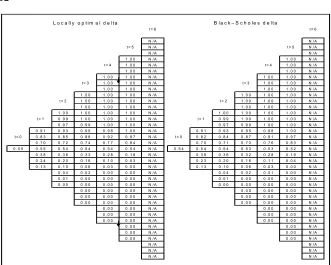
The locally optimal delta is easily computed from formula (15), be-cause we already know the values ofH in all nodes. Figure 5 compares

¯

θD_t with its continuous-time counterpart,

θBS_t =N



lnS/K+

³

r+σ₂2´(T₋t)

σ√T₋t



. (16)

3.3. Squared error process

The mean value process Ht represents the target value the hedging

portfolioVtis trying to achieve. It follows from Theorem 3 thatVt=Ht

minimizes the expected squared replication error as seen at time t,

EP t

h

(VT −HT)2 i

. The size of the error in the ideal case Vt = Ht is

measured by the squared error process ε2_t and is computed recursively as follows

ε2_t = EP_t hε2_t+1i+kt+1ESREPt (Ht+1) (17)

B l a c k – S c h o l e s d e l t a

t = 6 t = 6

N / A N / A

t = 5 N / A t = 5 N / A

N / A N / A

1 . 0 0 N / A 1 . 0 0 N / A t = 4 1 . 0 0 N / A t = 4 1 . 0 0 N / A 1 . 0 0 N / A 1 . 0 0 N / A 1 . 0 0 1 . 0 0 N / A 1 . 0 0 1 . 0 0 N / A t = 3 1 . 0 0 1 . 0 0 N / A t = 3 1 . 0 0 1 . 0 0 N / A 1 . 0 0 1 . 0 0 N / A 1 . 0 0 1 . 0 0 N / A 1 . 0 0 1 . 0 0 1 . 0 0 N / A 1 . 0 0 1 . 0 0 1 . 0 0 N / A t = 2 1 . 0 0 1 . 0 0 1 . 0 0 N / A t = 2 1 . 0 0 1 . 0 0 1 . 0 0 N / A 1 . 0 0 1 . 0 0 1 . 0 0 N / A 1 . 0 0 1 . 0 0 1 . 0 0 N / A 1 . 0 0 1 . 0 0 1 . 0 0 1 . 0 0 N / A 1 . 0 0 1 . 0 0 1 . 0 0 1 . 0 0 N / A t = 1 0 . 9 9 1 . 0 0 1 . 0 0 1 . 0 0 N / A t = 1 0 . 9 9 1 . 0 0 1 . 0 0 1 . 0 0 N / A 0 . 9 7 0 . 9 9 1 . 0 0 1 . 0 0 N / A 0 . 9 7 0 . 9 9 1 . 0 0 1 . 0 0 N / A 0 . 9 1 0 . 9 3 0 . 9 5 0 . 9 8 1 . 0 0 N / A 0 . 9 1 0 . 9 3 0 . 9 5 0 . 9 8 1 . 0 0 N / A t = 0 0 . 8 3 0 . 8 5 0 . 8 8 0 . 9 2 0 . 9 7 N / A t = 0 0 . 8 2 0 . 8 4 0 . 8 7 0 . 9 1 0 . 9 7 N / A 0 . 7 0 0 . 7 2 0 . 7 4 0 . 7 7 0 . 8 4 N / A 0 . 7 0 0 . 7 1 0 . 7 3 0 . 7 6 0 . 8 3 N / A 0 . 5 5 0 . 5 5 0 . 5 4 0 . 5 4 0 . 5 4 0 . 5 4 N / A 0 . 5 4 0 . 5 4 0 . 5 4 0 . 5 3 0 . 5 3 0 . 5 2 N / A 0 . 3 8 0 . 3 6 0 . 3 3 0 . 2 8 0 . 1 8 N / A 0 . 3 8 0 . 3 6 0 . 3 2 0 . 2 8 0 . 1 9 N / A 0 . 2 4 0 . 2 0 0 . 1 6 0 . 1 0 0 . 0 3 N / A 0 . 2 3 0 . 2 0 0 . 1 6 0 . 1 1 0 . 0 4 N / A 0 . 1 3 0 . 1 0 0 . 0 6 0 . 0 3 0 . 0 0 N / A 0 . 1 3 0 . 1 0 0 . 0 6 0 . 0 3 0 . 0 0 N / A 0 . 0 4 0 . 0 2 0 . 0 0 0 . 0 0 N / A 0 . 0 4 0 . 0 2 0 . 0 1 0 . 0 0 N / A 0 . 0 1 0 . 0 0 0 . 0 0 0 . 0 0 N / A 0 . 0 1 0 . 0 0 0 . 0 0 0 . 0 0 N / A 0 . 0 0 0 . 0 0 0 . 0 0 0 . 0 0 N / A 0 . 0 0 0 . 0 0 0 . 0 0 0 . 0 0 N / A 0 . 0 0 0 . 0 0 0 . 0 0 N / A 0 . 0 0 0 . 0 0 0 . 0 0 N / A 0 . 0 0 0 . 0 0 0 . 0 0 N / A 0 . 0 0 0 . 0 0 0 . 0 0 N / A 0 . 0 0 0 . 0 0 0 . 0 0 N / A 0 . 0 0 0 . 0 0 0 . 0 0 N / A 0 . 0 0 0 . 0 0 N / A 0 . 0 0 0 . 0 0 N / A 0 . 0 0 0 . 0 0 N / A 0 . 0 0 0 . 0 0 N / A 0 . 0 0 0 . 0 0 N / A 0 . 0 0 0 . 0 0 N / A 0 . 0 0 N / A 0 . 0 0 N / A 0 . 0 0 N / A 0 . 0 0 N / A 0 . 0 0 N / A 0 . 0 0 N / A

N / A N / A

N / A N / A

N / A N / A

L o c a l l y o p t i m a l d e l t a

Figure 5. Comparison between the locally optimal delta¯θDfrom equation (15) and the continuous-time Black—Scholes delta in (16).

The term ESREP_t (Ht+1) is the one-period Expected Squared

Replica-tion Error from hedging payoffHt+1 using the risk-free bank account

and the stock as basis assets

ESREP_t (Ht+1) = EPt ·³

RfHt+ ¯θ D

t St(Rt+1−Rf)−Ht+1 ´2¸

.

In our model with IID returns and non-stochastic interest rate process k becomes deterministic

kt=R2(_f T−t)bT−t= 0.9962T−t.

Recall from (12) that b = 1₋ (E

P

t [Rt+1−Rf])

2

EP

t[(Rt+1−Rf)2]. An econometrician

would interpret (E

P

t[Rt+1−Rf])

2

EP

t[(Rt+1−Rf)2]as the non-central R

2_{from the regression}

interpreted in terms of the market Sharpe RatioSR,

b= (1 + SR2)−1;

the quantity 1 ₋ √b _≈ 1₂SR2 measures the percentage increase in investor’s certainty equivalent wealth per unit of risk tolerance, see Chapter 3 in Cerný (2004).ˇ

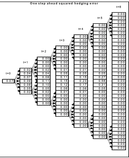
Figure 6 depicts the one-period expected squared hedging errors. Intuitively we know that options far in the money and far out of the money can be replicated perfectly. Indeed, we observe that the repli-cation error is the largest at the money and that it goes down to zero for very high and very low stock prices. There is a simple relationship between the one-step ahead expected squared hedging error and the optiongamma.This link is best seen by comparingESREP_t(Ht+1)with

formula (18) in Toft (1996) where transaction costs are ignored.

t= 6

0 .0 0

t= 5 0 .0 0

0 .0 0 0 .0 0 0 .0 0

t= 4 0 .0 0 0 .0 0

0 .0 0 0 .0 0 0 .0 0 0 .0 0 0 .0 0

t= 3 0 .0 0 0 .0 0 0 .0 0

0 .0 0 0 .0 0 0 .0 0 0 .0 0 0 .0 0 0 .0 0 0 .0 0

t= 2 0 .0 0 0 .0 0 0 .0 0 0 .0 0

0 .0 0 0 .0 0 0 .0 0 0 .0 0

0 .0 0 0 .0 0 0 .0 0 0 .0 0 0 .0 0

t= 1 0 .0 0 0 .0 0 0 .0 0 0 .0 0 0 .0 0

0 .0 0 0 .0 0 0 .0 0 0 .0 0 0 .0 0

0 .0 2 0 .0 2 0 .0 1 0 .0 1 0 .0 0 0 .0 0

t= 0 0 .0 4 0 .0 4 0 .0 5 0 .0 5 0 .0 5 0 .0 0

0 .0 7 0 .0 8 0 .1 1 0 .1 5 0 .2 7 0 .0 0

0 .0 7 0 .0 9 0 .1 1 0 .1 5 0 .2 3 0 .5 6 0 .0 0

0 .0 8 0 .1 0 0 .1 2 0 .1 7 0 .3 1 0 .0 0

0 .0 5 0 .0 5 0 .0 6 0 .0 6 0 .0 5 0 .0 0

0 .0 2 0 .0 2 0 .0 1 0 .0 1 0 .0 0 0 .0 0

0 .0 0 0 .0 0 0 .0 0 0 .0 0 0 .0 0

0 .0 0 0 .0 0 0 .0 0 0 .0 0 0 .0 0

0 .0 0 0 .0 0 0 .0 0 0 .0 0 0 .0 0

0 .0 0 0 .0 0 0 .0 0 0 .0 0 0 .0 0 0 .0 0 0 .0 0 0 .0 0 0 .0 0 0 .0 0 0 .0 0 0 .0 0 0 .0 0 0 .0 0 0 .0 0 0 .0 0 0 .0 0 0 .0 0 0 .0 0 0 .0 0 0 .0 0 0 .0 0 0 .0 0 0 .0 0 0 .0 0 0 .0 0 0 .0 0 0 .0 0 0 .0 0 0 .0 0

O n e s te p a h e a d s q u a r e d h e d g in g e r r o r

Figure 6. One-period expected squared hedging errors.

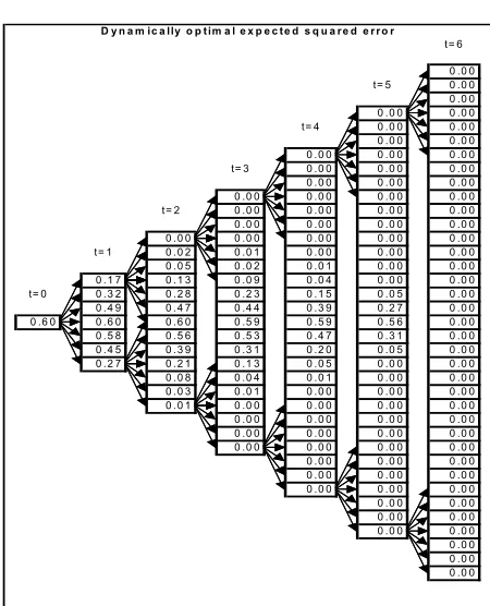
The total expected squared replication error ε2

t can be computed

recursively from (14). Numerical values are shown in Figure 7.

To summarize, if one sells one option at H0 = 2.32 and hedges

it optimally to maturity then one has entered a risky position with expected payoffzero and standard deviation ofε0 =

√

t= 6

0 .0 0

t= 5 0 .0 0

0 .0 0 0 .0 0 0 .0 0

t= 4 0 .0 0 0 .0 0

0 .0 0 0 .0 0 0 .0 0 0 .0 0 0 .0 0

t= 3 0 .0 0 0 .0 0 0 .0 0

0 .0 0 0 .0 0 0 .0 0 0 .0 0 0 .0 0 0 .0 0 0 .0 0

t= 2 0 .0 0 0 .0 0 0 .0 0 0 .0 0

0 .0 0 0 .0 0 0 .0 0 0 .0 0

0 .0 0 0 .0 0 0 .0 0 0 .0 0 0 .0 0

t= 1 0 .0 2 0 .0 1 0 .0 0 0 .0 0 0 .0 0

0 .0 5 0 .0 2 0 .0 1 0 .0 0 0 .0 0

0 .1 7 0 .1 3 0 .0 9 0 .0 4 0 .0 0 0 .0 0

t= 0 0 .3 2 0 .2 8 0 .2 3 0 .1 5 0 .0 5 0 .0 0

0 .4 9 0 .4 7 0 .4 4 0 .3 9 0 .2 7 0 .0 0

0 .6 0 0 .6 0 0 .6 0 0 .5 9 0 .5 9 0 .5 6 0 .0 0

0 .5 8 0 .5 6 0 .5 3 0 .4 7 0 .3 1 0 .0 0

0 .4 5 0 .3 9 0 .3 1 0 .2 0 0 .0 5 0 .0 0

0 .2 7 0 .2 1 0 .1 3 0 .0 5 0 .0 0 0 .0 0

0 .0 8 0 .0 4 0 .0 1 0 .0 0 0 .0 0

0 .0 3 0 .0 1 0 .0 0 0 .0 0 0 .0 0

0 .0 1 0 .0 0 0 .0 0 0 .0 0 0 .0 0

0 .0 0 0 .0 0 0 .0 0 0 .0 0 0 .0 0 0 .0 0 0 .0 0 0 .0 0 0 .0 0 0 .0 0 0 .0 0 0 .0 0 0 .0 0 0 .0 0 0 .0 0 0 .0 0 0 .0 0 0 .0 0 0 .0 0 0 .0 0 0 .0 0 0 .0 0 0 .0 0 0 .0 0 0 .0 0 0 .0 0 0 .0 0 0 .0 0 0 .0 0 0 .0 0

D y n a m ic a lly o p tim a l e x p e c te d s q u a r e d e r r o r

Figure 7. The smallest possible expected squared hedging error to maturity, ε2 t,

corresponding to a perfectly balanced hedging portfolio,Vt=Ht.

4. The variance-optimal measure

Theorem 2 does not use any duality theory and the only technical difficulty is tofind the self-preserving recursive structure (3), (4). Never-theless, a martingale measure, known as thevariance-optimal measure, emerges from the solution in equation (6).

Let us define

˜

m_{t|t−1 ≡}R_f2_t−1kt−E

P

t−1[kt∆Xt∗] ³

EP_t−1[kt∆Xt∆Xt∗] ´−1

kt∆Xt

kt−1

(18)

We notice that EP_t−1hm˜t|t−1 i

= 1by virtue of equation (5), and more-over m˜t|t−1 is Ft-measurable. Thereforem˜t|t−1 can be thought of as a

one-step conditional change of measure. The problem is that m˜_t|t−1 is

not necessarily strictly positive, and thus one has to be careful when defining conditional expectations.

We can define the density process

˜

and write

d ˜P

dP = ˜mT.

Since m˜_t|t−1can be equal to0with positive probability, the ratio m˜T

˜ mt is

not well defined. But if we formally agree that

˜

mT

˜

mt ≡

˜

mT|T−1. . .m˜t+1|t

then we can write

EP_t˜[X] = E

P

t [ ˜mTX]

˜

mt ≡

EP_t hm˜T|T−1. . .m˜t+1|tX i

(20)

as if P˜ were equivalent to P. Note that by Theorem 1 each of the

variables m˜_t+1|t is well defined. Thus although P˜ is a signed measure and generally not equivalent to P,equation (20) grants a well defined conditional expectation underP˜.

Another interesting property of P˜ is that it turns the discounted gain process into a martingale

EP_t˜₋₁[∆X_t∗]_≡EP_t−1hmt|t−1∆Xt∗ i

=R2_ft−1

×E

P

t−1[kt∆Xt∗]−EPt−1[kt∆Xt∗] ³

EP_t−1[kt∆Xt∆Xt∗] ´−1

EP_t−1[kt∆Xt∆Xt∗]

kt−1 = 0.

Finally, recursive application of equation (6) together with the law of iterated expectations imply

Ht

S0 t

= EP_t

"

˜

mT|T−1. . .m˜t+1|t

HT

S0 T

#

= EP_t˜

"

HT

S0 T

#

ˆ

x = H0= E

˜ P 0

"

HT

S_T0

#

. (21)

4.1. Special case: minimal martingale measure

When kt = EPt h

R2_ft. . . R2_fT−1i we obtain one-step conditional change of measure of the so-called minimal martingale measure. When the risk-free rate is non-stochastic the minimal change of measure becomes

ˆ

m_t|t−1 = 1−E

P

t−1[∆Xt∗] ³

EP_t−1[∆Xt∆Xt∗] ´−1

∆Xt

1₋EP_t−1[∆X_t∗]¡EP_t−1[∆Xt∆Xt∗] ¢−1

EP_t−1[∆Xt]

4.2. Variance-optimal measure and arbitrage

With P˜ being a martingale measure the equation (21) looks like a

no-arbitrage pricing formula, and therefore H0 is referred to by Schäl

(1994) as the fair hedging price of the contingent claim HT, while

Schweizer (1995) calls H0 approximation price. Schweizer correctly

ac-knowledges, however, that the termprice is misleading sinceH0 is not

necessarily a no-arbitrage price of HT.

A related point is that the variance-optimal measure exists even

when there is arbitrage among the basis assets. Take a simple binomial tree example with Rf = 1, no dividends, where St+1

St can only take

two values, +4 and +2 with equal probability 1₂. Since in both states the risky return is greater than the risk-free rate there is arbitrage. The model is actually complete, so there is only one candidate for the variance-optimal ‘probabilities’

4qup+ 2qdown = 1

qup+qdown = 1

qup = − 1 2

qdown = 3 2.

One can show that the hedging procedure described in Theorem 2 will go through fine, with kt = 0.1T−t. This means that mean-variance

hedging is not arbitrage-proof, in the sense that the algorithm described in Corollary 4 will not automatically come to a halt if there is arbitrage among the basis assets.

As an aside we highlight the result of Schachermayer (1993) who

showed that the minimal measure Pˆ (which in the above example is

equal to the variance-optimal measure P˜) may not exist even when there is no arbitrage. This would seem to contradict our Theorem 1, however, Schachermayer’s result has to do with integrability and we assumed away all integrability problems by taking Ω finite.

5. Comparison with previous studies

5.1. Definitions of variance-optimal measure

It follows from Section 4 that the natural definition of the variance-optimal measure P˜ is

d ˜P

wherem˜t|t−1 was given in equation (18). Let us see how this definition

relates to that of other authors, namely Schweizer (1995), Gourieroux et al. (1998), and Laurent and Pham (1999).

To simplify expression (23) let us define

at−1≡ ³

EP_t−1[kt∆Xt∆Xt∗] ´−1

EP_t−1[kt∆Xt], (24)

whereby the expression for the conditional change of measure becomes

˜

mt|t−1 =

R2

ft−1kt(1−a∗t−1∆Xt)

kt−1

. (25)

For the unconditional change of measure we then have

˜

mT = T Y

t=1

R2_ft−1kt(1−a∗t−1∆Xt)

kt−1

=

¡

S_T0¢2 k0

T Y

t=1

(1₋a∗_t−1∆Xt). (26)

Since by construction EP₀ [ ˜mT] = 1, an immediate consequence of the

above is

k0 = EP0 "_³

S_T0´2

T Y

t=1

(1₋a∗_t−1∆Xt) #

. (27)

Similarly, the fact that

EP_t hm˜t+1|tm˜t+2|t+1. . .m˜T|T−1 i

=

= EP_t          ˜

m_t+1|tEP_t+1   

m˜t+2|t+1. . .EPT−1 h

˜

m_T|T−1i

| {z }

=1

   

| {z }

=1          = 1 implies

kt= EPt

 

Ã

S_T0 S0 t

!2 _T

Y

j=t+1

(1₋a∗_j−1∆Xj)



Plugging this result back into equation (24) we have

at−1 =

 EP_t−1



∆Xt∆Xt∗EPt

 

Ã

S_T0 S0 t

!2 _T

Y

j=t+1

(1₋a∗_j−1∆Xj)

      −1

×EP_t−1

 ∆XtEPt

 

Ã

S_T0 S0 t

!2 _T

Y

j=t+1

(1₋a∗_j−1∆Xj)

    =  EP_t−1



∆Xt∆Xt∗ Ã

S0 T

S_t0

!2 _T

Y

j=t+1

(1₋a∗_j−1∆Xj)

 

 

−1

×EP_t−1

 ∆Xt

Ã

S_T0 S_t0

!2 _YT

j=t+1

(1₋a∗_j−1∆Xj)



. (29)

The above expression implies that for zero interest rate the process a coincides with the adjustment process β of Schweizer (1995). Further-more, Schweizer defines the variance-optimal measure P˜ as

d ˜P

dP =

QT

t=1(1−a∗t−1∆Xt)

EP 0

hQT

t=1(1−a∗t−1∆Xt) i,

and this definition by virtue of (27) coincides with our definition of the variance-optimal measure (26) when the interest rate is zero.

An alternative interpretation of formula (26) comes from the feed-back form (7) when we set HT = 0 and keepx= 1:

˜

θt−1 =−

V_t1₋,˜θ₁ S0

t−1

at−1, (30)

whereby it becomes clear that at = ˜at in Laurent and Pham (1999).

Here V_t1₋,˜θ₁ is interpreted as the optimal wealth from the self-financing

strategy that minimizes EP₀ hV_Tx,θi2 with initial wealth x = 1, ˜θ being the corresponding optimal investment strategy. From (1) we can write

V_t1,˜θ = Rft−1V1, ˜ θ

t−1+St0˜θt−1∆Xt

= Rft−1V1, ˜ θ t−1 ¡

1₋a∗_t−1∆Xt¢

and hence

V_T1,˜θ =

T Y

t=1

Rft−1(1−a∗t−1∆Xt) = (31)

= V_t1,˜θS

0 T

S_t0

T Y

j=t+1

Therefore, from (31) and (26) the variance-optimal change of measure can be expressed equivalently as

˜

mT =

S_T0V_T1,˜θ k0

= S 0 TV

1,˜θ T

EP₀

·

S_T0V_T1,˜θ

¸

as in Gourieroux et al. (1998), equation (4.4). One can use (32) to write (28) as

kt=

EP t

·

V_T1,˜θS0 T ¸

V_t1,˜θS0 t

.

On the other hand equation (4.7) in Laurent and Pham (1999) implies

jt=

V_t1,˜θS_t0

EP_t

·

V_T1,˜θS_T0

¸

and hence our process kis the same as their process i_≡ 1_j.

5.2. Feedback form

Schweizer (1995)finds a feedback solution of the following form

θD_t = ρ_t−β_tVH0,θD

t (33)

ρ_t = E

P t−1

h

∆XtQTj=t+1 ³

1₋β_j∆Xj ´

HT i

EP t−1

·

(∆Xt)2QTj=t+1 ³

1₋β_j∆Xj

´2¸. (34)

assuming Rft= 1.To verify that (33) is equivalent to (7) we have to

show that ρ_t =³EP_t−1h(∆Xt)2kt i´−1

EP_t−1[kt∆XtHt]. First we employ

the law iterated expectations

ρ_t =

EP_t−1h∆XtQTj=t+1 ³

1₋β_j∆Xj ´

HT i

EP_t−1

·

(∆Xt)2QTj=t+1 ³

1₋β_j∆Xj ´2¸

=

EP_t−1h∆Xt h

EP_t QT_j=t+1³1₋β_j∆Xj ´

HT ii

EP_t−1

·

(∆Xt)2EPt ·

QT j=t+1

³

using the fact that ∆Xt isFt-measurable. From Lemma 3 in Schweizer

(1996) one has

EP_t  

T Y

j=t+1 ³

1₋β_j∆Xj ´2

 = EP_t

 

T Y

j=t+1 ³

1₋β_j∆Xj ´

. (35)

On the other hand, equation (28) in this paper claims

kt= EPt

 

T Y

j=t+1 ³

1₋β_j∆Xj ´

. (36)

Thus we have

ρ_t = E

P t−1

h

kt∆XtEPt h

HTQTj=t+1 kj

kj−1

³

1₋β_j∆Xj ´ii

EP_t−1h(∆Xt)2kt i

= E

P t−1

h

kt∆XtEPt h

˜

mt|t−1. . .m˜T|T−1HT ii

EP_t−1h(∆Xt)2kt i

= E

P

t−1[kt∆XtHt]

EP t−1

h

(∆Xt)2kt i

as required by virtue of (6), (18) and (25).

The continuous time solution in feedback form was obtained for the first time in Schweizer (1992) under the assumption of constant opportunity set, which implies P˜ = ˆP. A general proof for continuous semimartingales was given in Gourieroux, Laurent, and Pham (1998) and Rheinländer and Schweizer (1997). Let us rewrite (7) in a more familiar form, similar to equation (0.1) in Rheinländer and Schweizer (1997).

ˆ

θt−1 = − h

EP_t−1kt∆Xt∆Xt∗ i−1

EP_t−1kt∆Xt

 V

H0,ˆθ

t−1

S_t0₋₁ − Ht

S_t0

 =

= Rft−1at−1

VH0,ˆθ

t−1 −Ht−1

S_t0₋₁ +

+³EP_t−1[kt∆Xt∆Xt∗] ´−1

EP_t−1

·

kt∆Xt∆

Ht

S0 t ¸

It follows from the results of Rheinländer and Schweizer (1997) that for continuous gain process the second term can be interpreted as the

of HT

S0 T

under P .˜ This is essentially made possible by the fact that for continuous processes the randomness ofkin the above formula vanishes and that both processes X and _SH0 are martingales under P. In jump-˜

diffusion limit, however, such interpretation is no longer possible, even ifkt is deterministic.

It seems more difficult to relate directly our formula (7) to the con-tinuous time result of Gourieroux et al. (1998), Theorem 5.1. We can only refer to Rheinländer and Schweizer (1997) who show the equiva-lence between their equation (0.1) and the Theorem 5.1 of Gourieroux et al. (1998).

5.3. Continuous limit

It is interesting to see what happens to the solution in continuous time

limit if we assume that all processes become Itô processes. When X

is a Markov process this procedure can be formalized using the locally consistent Markov chain approximations championed in Kushner and Dupuis (2001).

Assume that the stochastic differential equation for the discounted gain process satisfies

Xt+dt−Xt≡dXt=µdt+σdBt,

and the processk follows

dkt=µkdt+σkdBt.

The continuous-time counterpart of equation (5) reads

kt= (1 +rtdt)2

×

µ

EP_t [kt+dt]−EPt [kt+dtdXt∗] ³

EP_t [kt+dtdXtdXt∗] ´₋1

EP_t [kt+dtdXt] ¶

.

(37)

From the Itô’s lemma we have

EP_t [kt+dt] = kt+µkdt+o(dt)

EP_t [kt+dtdXt] = ktµdt+σσ∗kdt+o(dt)

EP_t [kt+dtdXtdXt∗] = ktσσ∗dt+o(dt),

and collecting the dt terms in (37) we obtain

0 = 2kr+µ_k−(kµ+σσ∗_k)∗(kσσ∗)−1(kµ+σσ∗_k)

0 = 2r+µk

k −

µ

µ+σσ

∗

k

k

¶∗

(σσ∗)−1

µ

µ+σσ

∗

k

k

¶

Similarly, from (30) we have

a= (σσ∗)−1

µ

µ+σσ

∗

k

k

¶

.

To see the market price of risk defining the variance-optimal measure we have to look at the continuous time limit of equation (18),

˜

mt+dt|t= (1 +rtdt)2

×

kt+dt−EPt [kt+dtdXt∗] ³

EP

t [kt+dtdXtdXt∗] ´−1

kt+dtdXt

kt

=

= 1 +

µ_σ

k

k

³

I₋σ∗(σσ∗)−1σ´₋µ∗(σσ∗)−1σ

¶

dB.

Taking into account that m˜t+dt|t = m˜_mt+dt_˜t we can rearrange the above

equation to obtain

d ˜mt= ˜mt

½_σ

k

k

³

I₋σ∗(σσ∗)−1σ´₋µ∗(σσ∗)−1σ

¾

dB

whereby we identify

˜

λ_{≡ −}hI₋σ∗(σσ∗)−1σiσ

∗

k

k +σ

∗_(σσ∗₎−1_µ

as the variance-optimal market price of risk. Recall that the variable

λ_≡σ∗(σσ∗)−1µ

is known as the minimal market price of risk. There are three interesting special cases:

1. kis non-stochastic. In this caseσk= 0and consequently

˜

λ = λ

a = (σσ∗)−1µ

2. dkis perfectly correlated with the gain processdX.In this case

h

I₋σ∗(σσ∗)−1σiσ∗_k= 0

and therefore

˜

λ=λ,

3. dkis uncorrelated with the gain processdX (σσ∗_k= 0). Then

˜

λ=λ₋σ

∗

k

k and from (38) we have

0 = 2r+µk

k −µ

∗_(σσ∗₎−1

µ= 2r+µk

k −λ

2_.

Note that the Markov chain approximation results coincide with the rigorously derived results of Laurent and Pham (1999), who in the cases 2. and 3. are able to provide more explicit characterization of the processk (called iin their paper).

6. Conclusion

This paper presents a dynamic programming solution to the general mean-variance hedging problem in discrete time. Our analysis shows that in discrete time a natural solution exists which does not require the use of either variance-optimal martingale measure or duality theory. Comparing the continuous time limit of our results with the results obtained for continuous semimartingales by martingale and duality methods we observe that our solution gives good explicit characteri-zation of the variance-optimal market price of risk, however, it is not as detailed as the results of Laurent and Pham (1999). One merit of our solution is that it provides the kind of minimalistic recursive structure suitable for computer implementation, and that it offers a simple non-technical context in which the results of previous studies are easier to analyze and understand. The results presented here are a natural stepping stone to the analysis of hedging with discontinuous price processes.

Appendix

A. Proof of Theorems 2 and 3

1) Linear independence of basis assets meansθ∗_t−1∆Xt= 0a.s.⇒θ∗t−1 = 0 where θ∗_t−1 is _Ft−1-measurable. By contradiction assume that the

matrixEP_t−1[kt∆Xt∆Xt∗]is singular at a particular information node at

t₋1. Then there isθ∗_{t−1 6}= 0such that

0 = θ∗_t−1EP_t−1[kt∆Xt∆Xt∗]θt−1 = EP_t−1·³θ_t∗₋₁pkt∆Xt

at that node, which is only possible if θ∗_t−1√kt∆Xt = 0 at the node

in question. Since by assumption √kt > 0 a.s., we have θ∗t−1∆Xt = 0

and from the linear independence of random variables ∆Xt it follows

that θ∗_t−1 = 0 which contradicts θ∗_{t−1 6}= 0. Hence EP_t−1[kt∆Xt∆Xt∗] is

invertible at every node of the information set_Ft−1.

2) We wish tofind the optimal controlx_∈F0,θi∈Fi,i= 0,1, . . . , T−

1,to minimize

min

x,θ0,...,θt−1 EP₀

 kt

Ã

S0_t

Ã

V₀x,θ+

t−1 X

i=0

θi∆Xi+1 !

−Ht

!2

.

given thatkt>0andHtareFt-measurable and exogenous in the sense

of Definition 1. Bellman’s principle of optimality dictates

min

x,θ0,...,θt−1 EP₀

·

kt ³

V_tx,θ₋Ht ´2¸

=

= min

x,θ0,...,θt−2 EP₀

·

min θt−1

EP_t−1

·

kt ³

V_tx,θ₋Ht ´2¸¸

=

= min

x,θ0,...,θt−2 EP₀

·

min θt−1

EP_t−1

·

kt ³

Rft−1Vtx,−θ1+St0θt−1∆Xt−Ht ´2¸¸

,

where the last equality follows from the definition of self-financing strategy (1).

The partial problem

Jt−1,min θt−1

EP_t−1

·

kt ³

Rft−1Vtx,−θ1+St0θt−1∆Xt−Ht ´2¸

(39)

is simply a least squares regression. Let us recall that the abstract problem

ˆ

U = min

β E [Y +X

∗_β]2

has the following solution

ˆ

β = ₋(E [XX∗])−1E [XY] ˆ

U = EhY2i₋(E [XY])∗(E [XX∗])−1E [XY],

provided that the random variables X are linearly independent. Thus the problem (39) is solved by setting

ˆ

U = Jt−1

Y _≡ pkt ³

Rft−1Vtx,−θ1−Ht ´

X _≡ pkt∆Xt

whereby, after collecting all the powers of V, we obtain

Jt−1 = kt−1 ³

V_tx,₋θ₁₋Ht−1 ´2

+ EP_t−1hktHt2 i

−kt−1Ht2−1−

−³EP_t−1[kt∆XtHt] ´∗³

EP_t−1[kt∆Xt∆Xt∗] ´−1

EP_t−1[kt∆XtH(40)t]

θD_t−1=₋ 1

S_t0

³

EP_t−1[kt∆Xt∆Xt∗] ´₋1

EP_t−1hkt∆Xt ³

Rft−1Vx,θ

D

t−1 −Ht ´i

with kt−1, Ht−1 defined in (5), (6).

3) It remains to be shown that the processHt−1 is well defined, that

is kt−1 >0a.s. By assumption kt>0a.s. Note from (5) thatkt−1 can

be written equivalently as

kt−1 =R2ft−1EPt−1 ·³p

kt−θ∗ p

kt∆Xt ´2¸

, (41)

with θ∗ = EP_t−1[kt∆Xt∗] ³

EP_t−1[kt∆Xt∆Xt∗] ´−1

. We continue the proof by contradiction: suppose that kt−1 = 0 at a particular node. From

(41) this is only possible if √kt−θ∗√kt∆Xt= 0 a.s. for a conditional

distribution at this node. Since by assumption √kt > 0 it must be

that 1 = θ∗∆Xt for the conditional distribution at this node, which

contradicts our assumption of no arbitrage at that node. Hence it must be that kt−1 >0 a.s.

4) By induction assumption kt and Ht are exogenous. Clearly, the

conditional expectation of an exogenous variable is still exogenous, and any function of exogenous variables is again exogenous. Since the formulae (5), (6) only involve functions and conditional expectations of exogenous variables it follows that kt−1 and Ht−1 are exogenous. The

same reasoning implies that the last three terms in equation (40) are exogenous, that is the problem

min

x,θ0,...,θt−1 EP₀

·

kt ³

V_tx,θ₋Ht ´2¸

=

= EP₀ hktHt2−kt−1Ht2−1−

−³EP_t−1[kt∆XtHt] ´∗³

EP_t−1[kt∆Xt∆Xt∗] ´−1

EP_t−1[kt∆XtHt] ¸

+

+ min

x,θ0,...,θt−2 EP₀

·

kt−1 ³

V_tx,₋θ₁₋Ht−1 ´2¸

has the same optimal controls as the problem

min θ0,...,θt−2

EP₀

·

kt−1 ³

V_tx,₋θ₁₋Ht−1 ´2¸

which completes the proof of Theorem 2.

4) As a by-product of the above calculation we have learnt that

min θt−1

EP_t−1

·

kt ³

V_tx,θ₋Ht ´2¸

=kt−1 ³

V_tx,₋θ₁₋Ht−1 ´2

+ ESREP_t−1(Ht),

(42) where the one-step ahead expected squared replication error is given by

ESREP_t−1(Ht)≡EPt−1 h

ktHt2 i

−kt−1Ht2−1

−³EP_t−1[kt∆XtHt] ´∗³

EP_t−1[kt∆Xt∆Xt∗] ´−1

EP_t−1[kt∆XtHt].

A simple manipulation demonstrates the identity

ESREP_t−1[Ht] = EPt−1 ·

kt ³

Rft−1Ht−1+St0 ³

¯

θD_t−1´∗∆Xt−Ht ´2¸

,

where ¯θD_t is given by (8).

5) A recursive application of (42) starting from t=T gives

min θt−1

EP_t−1

·

kT ³

V_Tx,θ₋HT ´2¸

=kt−1 ³

V_tx,₋θ₁₋Ht−1 ´2

+ε2_t−1

where εis given recursively

ε2_t−1 = EP_t−1hε2_ti+ ESREP_t−1[Ht],

εT = 0.

which completes the proof of Theorem 3.

References

Bertsimas, D., L. Kogan, and A. W. Lo (2001). Hedging deriva-tive securities and incomplete market: An ²-arbitrage approach.

Operations Research 49(3), 372—397.

ˇ

Cerný, A. (1999). Currency crises: Introduction of spot speculators.

International Journal of Finance and Economics 4(1), 75—89.

ˇ

Cerný, A. (2002). Derivatives without differentiation: Optimal hedg-ing on Markov chains. Technical report, Imperial College Man-agement School.

ˇ

Cerný, A. (2004). Mathematical Techniques in Finance: Tools for

Duffie, D. and H. Richardson (1991). Mean—variance hedging in continuous time.Annals of Applied Probability 1, 1—15.

Föllmer, H. and M. Schweizer (1991). Hedging of contingent claims under incomplete information. In M. H. A. Davis and R. J. El-liott (Eds.),Applied Stochastic Analysis, pp. 389—414. New York: Gordon and Breach.

Frey, R. and A. Stremme (1997). Market volatility and feedback effects from dynamic hedging. Mathematical Finance 7(4), 351— 374.

Gourieroux, C., J.-P. Laurent, and H. Pham (1998). Mean-variance hedging and numéraire.Mathematical Finance 8(3), 179—200.

Kushner, H. J. and P. Dupuis (2001). Numerical Methods for

Sto-chastic Control Problems in Continuous Time(2nd ed.). Springer Verlag.

Laurent, J. P. and H. Pham (1999). Dynamic programming and mean-variance hedging.Finance and Stochastics 3(1), 83—110.

Rheinländer, T. and M. Schweizer (1997). On L2 projections on a space of stochastic integrals. Annals of Probability 25(4), 1810— 1831.

Schachermayer, W. (1993). A counterexample to several problems in the theory of asset pricing.Mathematical Finance 3, 217—229.

Schäl, M. (1994). On quadratic cost criteria for option hedging.

Mathematics of Operations Research 19(1), 121—131.

Schweizer, M. (1992). Mean-variance hedging for general claims.The Annals of Applied Probability 2(1), 171—179.

Schweizer, M. (1995). Variance-optimal hedging in discrete time.

Mathematics of Operations Research 20(1), 1—32.

Schweizer, M. (1996). Approximation pricing and the

variance-optimal martingale measure. The Annals of Probability 24(1),

206—236.

Schweizer, M. (1998). Risky options simplified.International Journal of Theoretical and Applied Finance 2(1), 59—82.

Toft, K. B. (1996). On the mean-variance tradeoff in option

repli-cation with transactions costs. The Journal of Financial and