Lattice Boltzmann model for thermal transpiration

A lattice Boltzmann model for thermal transpiration

G. H. Tang∗

Computational Science and Engineering Department,

STFC Daresbury Laboratory, Warrington, WA4 4AD, United Kingdom

Y. H. Zhang†

Department of Mechanical Engineering,

University of Strathclyde, Glasgow, G1 1XJ, United Kingdom

X. J. Gu, R. W. Barber, and D. R. Emerson

Computational Science and Engineering Department,

STFC Daresbury Laboratory, Warrington, WA4 4AD, United Kingdom

(Dated: September 18, 2008)

Abstract

The conventional Navier-Stokes-Fourier equations with no-slip boundary conditions are unable to capture the phenomenon of gas thermal transpiration. While kinetic approaches such as the direct simulation Monte Carlo (DSMC) method and direct solution of the Boltzmann equation can predict thermal transpiration, these methods are often beyond the reach of current com-puter technology, especially for complex three-dimensional flows. In this brief report, we present a new computationally efficient nonequilibrium thermal lattice Boltzmann model for simulating temperature-gradient-induced flows. The excellent agreement between our model and kinetic ap-proaches demonstrates the capabilities of the proposed lattice Boltzmann method.

PACS numbers: 05.10.-a, 47.45.-n, 47.61.-k

I. INTRODUCTION

In 1879, Osborne Reynolds discovered that a gas will move along a solid surface due to inequalities of temperature and called the phenomenonthermal transpiration[1]. In the same year, Maxwell [2] independently developed a theory to explain this effect. The phenomenon of thermal transpiration (or thermal creep [3]) has recently been used to develop a MEMS-based multi-stage Knudsen compressor [4, 5] where the gas moves from a cold chamber to a hot chamber and builds up a pressure difference across the compressor element. Thermal creep occurs in the opposite direction to the tangential heat flux, i.e., the flow is in the direction of increasing temperature.

The physical explanation of thermal creep has been presented by Sone [6]. It is assumed that equal numbers of molecules arrive at the wall from the hot and cold regions. Molecules arriving from the hot region will have, on average, a higher velocity than those arriving from the cold region. Since the molecules are reflected diffusively at the wall, the resultant force on the wall due to the molecular collisions acts towards the cold region. An equal and opposite force is felt by the gas molecules giving rise to a flow towards the hot region. Once the fluid starts to creep along the wall, the moving fluid layer interacts with the stagnant fluid layers adjacent to it, inducing a boundary layer.

II. NONEQUILIBRIUM THERMAL LATTICE BOLTZMANN MODEL

Conventional LB models are unable to capture nonlinear constitutive behavior close to a solid surface since they only retain velocity terms up to 2nd-order in the Hermite expansion of the equilibrium distribution function, as reported by Shan et al. [7]. However, this is not sufficient even for isothermal flows and it is usually necessary to retain terms up to 4th-order in the Hermite expansion. Moreover, to describe nonequilibrium physics beyond the level of the NSF equations, it is necessary to consider terms up to 5th-order in the Hermite expansion. Inevitably, this leads to a large number of discrete velocities which increases the computational cost and may give rise to numerical stability problems.

To overcome these difficulties, we make use of the different relaxation rates for momen-tum and energy, and propose a different energy density distribution function g to describe the evolution of the temperature field, as suggested by Heet al. [8] for no-velocity-slip and no-temperature-jump hydrodynamics. Using this approach, it is only necessary to retain up to the 3rd-order moments of the energy density distribution function in order to describe heat fluxes beyond the NSF level. As a consequence, our previously reported nonequilib-rium isothermal lattice Boltzmann model [9] should be sufficiently accurate to describe the evolution of the velocity field. In the present approach, as well as solving the evolution equation for the particle number density, we solve an additional equation for the energy density distribution function. The model relates the energy density distribution function to the number density distribution function via a flexible Prandtl number.

The evolution equation for the velocity field has previously been described by Zhang et al. [10]:

fk(x+ekδt, t+δt)−fk(x, t) =−

1

τ[fk(x, t)−f

eq

k (x, t)] +δt

(eki−ui)Fi

c2

sρ

f_keq(x, t), (1)

where fk is the distribution function for the number density at position x and time t, fkeq

is the corresponding distribution function at equilibrium, eki is the lattice velocity, ui is the

macroscopic velocity, cs is the sound speed of the lattice fluid, ρ is the density, τ is the

nondimensional relaxation time for the number density distribution function, and δt is the time step. The kinematic viscosity is calculated from ν= (τ₋0.5)c2

sδt. Following Heet al.

[8], the energy density evolution equation is given by

wheregkis the distribution function for the energy density at positionxand timet,gkeqis the

corresponding distribution function at equilibrium, and τt is the nondimensional relaxation

time for the energy density distribution function. The thermal diffusivity is given by α = (τt−0.5)c2sδt and the Prandtl number is determined from Pr = (τ−0.5)/(τt−0.5) [10, 11].

Viscous heating effects have been neglected in the present model since they are usually insignificant in low speed gas flows in micro/nano-devices.

Following the spirit of rational number approximation [12], we have developed a lattice Boltzmann isothermal model beyond the level of the Navier-Stokes equations [9]. For a two-dimensional, thirteen-velocity lattice model (D2Q13) [9], the lattice velocities are given by

e0 = 0,

ek =

"

cos (k−1)π 2

!

,sin (k−1)π 2

!#

c , k = 1₋4,

ek =

"

cos (k−5)π

2 +

π

4

!

,sin (k−5)π

2 +

π

4

!#√

2c , k = 5₋8, (3)

ek =

"

cos (k−1)π 2

!

,sin (k−1)π 2

!#

2c , k = 9₋12,

where c= √2RT and R is the gas constant. The equilibrium distribution function can be expressed as:

f_keq =ρωk

"

1 + ekiui

c2

s

+(ekiui) 2

2c4

s

− uiui 2c2

s

+(ekiui) 3

2c6

s

−3(ekiui)(uiui) 2c4

s

#

, (4)

ω0 = 3

8; ωk = 1

12 , k= 1−4 ; ωk = 1

16 , k= 5−8 ; ωk= 1

96 , k = 9−12.

The sound speed of the lattice fluid is given by c2

s = c2/2. The same D2Q13 lattice model

is used to solve the evolution equation for the energy density distribution function. At equilibrium, the energy density is given by geq_k = ǫf_keq, where ǫ = DRT /2 and D is the number of physical dimensions [10].

determined as follows:

τ = λ

λ0

ρref

ρ ( T Tref

)ω−0.5

rπ

8

c cs

Kn0NL+

1

2, (5)

whereNL =L/δy is the number of lattices over the characteristic lengthL,δy is the lattice

spacing, ρref is the density at the reference temperature Tref, and Kn0 is the Knudsen number based on the mean free path λ0 evaluated from λ0 = (µ0/p)

q

πRT /2, where p is the pressure and µ0 is the dynamic viscosity. The coefficient, ω, depends on the molecular interaction model, with ω = 0.5 for hard sphere interactions and ω = 1 for Maxwellian interactions. The local mean free path ratio, λ/λ0, can be solved separately depending on the specific geometric conditions [13–15]. The thermal relaxation time is determined from

τt= (τ −0.5)/Pr+0.5.

In this work, a kinetic boundary condition with a diffuse scattering kernel is employed. The unknown reflected distribution function fk on the wall can be determined from the

incident distribution function fk′ as follows [16]:

fk(x, t+δt) =

X

(ek′−uw)·n<0

|(ek′−u_w)·n|f_k′(x, t+δt)

X

(ek−uw)·n>0

|(ek−uw)·n|fkeq(x, ρw,uw)

fkeq(x, ρw,uw), (6)

where uw and ρw are the velocity and density at the wall, respectively, and n is the unit

normal. The above Maxwellian diffuse reflection at the wall assumes that the reflected particles are in thermal equilibrium with the wall. The reflected energy density distribution can therefore be related to the reflected number density distribution as follows [10]:

gk =

DR

2 Twfk, (7)

where Tw is the temperature of the wall.

III. RESULTS AND DISCUSSION

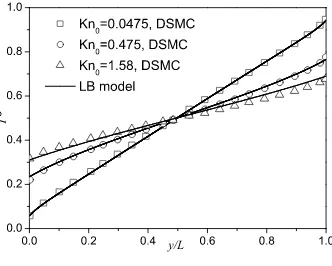
T∗ _{= (T −T}

1)/(T2 −T1). Figure 1 clearly shows that the temperature jump at the wall increases with Knudsen number. At low Kn, the temperature profile is almost linear but becomes increasingly nonlinear at higher Knudsen numbers. It can be seen that the LB model is in good agreement with the DSMC data in both the slip and transition regimes.

0.0 0.2 0.4 0.6 0.8 1.0

0.0 0.2 0.4 0.6 0.8 1.0

T

*

y/L

Kn

0

=0.0475, DSMC

Kn

0

=0.475, DSMC

Kn

0

=1.58, DSMC

LB model

FIG. 1: Nondimensional temperature profiles for rarefied Fourier flow between two parallel plates. The symbols represent the DSMC data presented by Gallis et al. _[17].

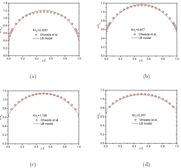
The second test case considers thermal creep flow between two parallel plates separated by a distance, L. Figure 2 shows the normalized velocity profiles across the channel at various Knudsen numbers and compares the results from our lattice Boltzmann model against the data obtained by Ohwada et al. [18] using a direct solution of the linearized Boltzmann equation. It can be seen that our LB model is in very good agreement with the solution from the linearized Boltzmann equation, indicating that the proposed model can capture thermal transpiration phenomena in the slip and transition regimes. To the best of the authors’ knowledge, this is the first successful attempt at modeling thermal transpiration using a lattice Boltzmann approach. Since the proposed method has a computational efficiency comparable to a Navier-Stokes solver, it offers a practical simulation tool for nonequilibrium thermal flows in industrially-relevant geometries.

IV. CONCLUSIONS

0.0 0.2 0.4 0.6 0.8 1.0 0.0 0.2 0.4 0.6 0.8 1.0 1.2 1.4 u / u m y/L Kn 0 =0.2257

Ohwada et al. LB m odel

0.0 0.2 0.4 0.6 0.8 1.0

0.0 0.2 0.4 0.6 0.8 1.0 1.2 u / u m y/L Kn 0 =0.677

Ohwada et al. LB m odel

(a) (b)

0.0 0.2 0.4 0.6 0.8 1.0

0.0 0.2 0.4 0.6 0.8 1.0 1.2 u / u m y/L Kn 0 =1.128

Ohwada et al. LB m odel

0.0 0.2 0.4 0.6 0.8 1.0

0.0 0.2 0.4 0.6 0.8 1.0 1.2 u / u m y/L Kn 0 =2.257

Ohwada et al. LB m odel

(c) (d)

FIG. 2: Velocity profiles for thermal creep flow between two parallel plates at (a) Kn0 = 0.2257, (b) Kn0 = 0.677, (c) Kn₀ = 1.128, and (d) Kn₀ = 2.257. The symbols represent the solution of the linearized Boltzmann equation presented by Owhada et al. _{[18] and the velocities have been}

normalized by the mean velocity in the channel,u_m.

V. ACKNOWLEDGMENTS

The authors would like to thank Dr. Michael Gallis of Sandia National Laboratories for kindly providing the DSMC data. We would also like to thank Professor Jason Reese from the University of Strathclyde for the helpful discussions. This work was financially supported by the UK Engineering and Physical Sciences Research Council (EPSRC) under grants EP/D07455X/1 and EP/F028865/1. Additional support was provided by EPSRC under the auspices of Collaborative Computational Project 12.

[1] O. Reynolds, Phil. Trans. R. Soc. London170, 727 (1879). [2] J. C. Maxwell, Phil. Trans. R. Soc. London 170, 231 (1879).

[3] E. H. Kennard, Kinetic Theory of Gases, McGraw-Hill New York and London (1938). [4] E. P. Muntz, Y. Sone, K. Aoki, S. Vargo, and M. Young, J. Vac. Sci. Technol. A 20, 214

(2002).

[5] Y. L. Han, E. P. Muntz, A. Alexeenko, and M. Young, Nanoscale Microscale Thermophys. Eng. 11, 151 (2007).

[6] Y. Sone, Annu. Rev. Fluid Mech.32, 779 (2000).

[7] X. W. Shan, X. F. Yuan, and H. D. Chen, J. Fluid Mech.550, 413 (2006). [8] X. Y. He, S. Chen, and G. D. Doolen, J. Comput. Phys. 146, 282 (1998). [9] G. H. Tang, Y. H. Zhang, and D. R. Emerson, Phys. Rev. E77, 046701 (2008). [10] Y. H. Zhang, X. J. Gu, R. W. Barber, and D. R. Emerson, EPL77, 30003 (2007). [11] Y. Shi, T. S. Zhao, and Z. L. Guo, Phys. Rev. E70, 066310 (2004).

[12] S. S. Chikatamarla and I. V. Karlin, Phys. Rev. Lett.97, 190601 (2006). [13] G. H. Tang, Y. H. Zhang, X. J. Gu, and D. R. Emerson, EPL 83, 40008 (2008). [14] D. W. Stops, J. Phys. D: Appl. Phys.3, 685 (1970).

[15] Z. L. Guo, B. C. Shi, and C. G. Zheng, EPL80, 24001 (2007). [16] S. Ansumali and I. V. Karlin, Phys. Rev. E 66, 026311 (2002).