Intelligent techniques for dynamic and transient analysis of multi stage desalination plant

City, University of London Institutional Repository

Citation: Abdelbary, A.F. (1997). Intelligent techniques for dynamic and transient analysis of multi stage desalination plant. (Unpublished Doctoral thesis, City University London)

This is the accepted version of the paper.

This version of the publication may differ from the final published version.

Permanent repository link: http://openaccess.city.ac.uk/7716/

Link to published version:

Copyright and reuse: City Research Online aims to make research outputs of City, University of London available to a wider audience. Copyright and Moral Rights remain with the author(s) and/or copyright holders. URLs from City Research Online may be freely distributed and linked to.

City Research Online: http://openaccess.city.ac.uk/ [email protected]

INTELLIGENT TECHNIQUES FOR

DYNAMIC AND TRANSIENT ANALYSIS OF

MULTI STAGE DESALINATION PLANT

by

Ayman Fahmy Abdelbary

This thesis submitted for the degree of

Doctor of Philosophy

at

Department of Electrical, Electronics and Information Engineering

City University

London

UK

Thesis Summary

This thesis is concerned with dynamic and transient analysis of MSF

desalination plants. The technique is developed using artificial neural

networks (ANN) approach for the purpose of prediction, analysis, modelling,

and control of MSF desalination plant. The applicability of the method to

predict an approximation of the transient operating conditions as well as the

control action are shown satisfactory. The network architecture and learning

algorithm are developed based on the Multilayered Feed forward Networks

(MFN) with the Back Propagation (BP) learning algorithm.

It was shown that

the approach could intelligently capture the dynamics of the system.

An

improved technique is developed for the BP learning algorithm based on

Global Error Node Evaluation (GENE)

approach for MFN to retains the

function approximation requirements for a nonlinear dynamic behaviour.

However, by using this approach considerable improvement for the

generalization capability could be obtained for the case study under

consideration. The technique provides the necessary dynamic learning

behaviour required for MFN. This approach appears to be effective for the

input - output dynamic modelling of complex process systems and therefore

on-line adaptation is possible (when the characteristic of the system is

changing or when more test data are available for another operating range).

The developed algorithm is used for the development and validation of an

elnpirical multi-controller structure for MSF desalination plant. Satisfactory

results are obtained from practical examples with the additional training

ability.

Summary of Original Contributions

To the best knowledge of the author, the following portion of the thesis is

considered as the original contributions:

1.

Improvement of the Back Propagation learning capability for Multi

Layered Feed forward Networks using GENE approach.

2.

Learning System Dynamics for MIMO using the MFN.

3.

Applicability of using the Artificial Neural Network for assisting the

modelling control problems found in MSF desalination process.

Part of the work described in this thesis is reported in the following

publications:

1

Abdulbary A. F., L.L. Lai, D.M.K. Al-Gobaisi, "Application of Neural

Network to Controlling and Modelling of a MSF Desalination Plant",

Thirteen IASTED Int. Conf. MODELLING, IDENTIFICATION AND

CONTROL, Feb., 21-23, 1994, Grindelwald, Switzerland, pp. 256-259

2

A F Abdelbary, L L Lai, D M K AlGobaisi and A Husain, "Experience

of using the neural network approach for identification of MSF

desalination plants" Desalination, 92 (1993) Elsevier Science Publishers

B.V., Amsterdam, pp. 323-331

3

Abdulbary A. F., L L Lai, and D M K Al-Gobaisi, "Application of a

connectioinest Model to controlling a MSF Desalination Plant" ,

Proceeding of 3rd IEEE Conference On Control Applications, Aug.

1994, Glasgow, UK, Vol 3, pp. 1821-1822.

4

Abdulbary A. F, L L Lai, K.V. Reddy, A. Husain, and D M K

Al-Gobaisi", Neural Networks as Efficient Tools of Simulation",

Proceeding of IDA World Congress On Desalination and Water Reuse,

Nov. 1995, Abu Dhabi, UAE, Vol IV pp. 361-374.

5

Abdulbary A. F., L L Lai, A. Husain, and D M K Al-Gobaisi, "

An

Introduction to Intelligent Control of Desalination Processes Using

Neural Networks",

Proceeding of

IDA World Congress On

Desalination and Water Reuse, Nov. 1995, Abu Dhabi, UAE, Vol I, pp

317.

ACKNOWLEDGMENTS

This research work was carried out in the Water and Electricity Department of Abu Dhabi. and at City University of London.

The author would like to thank his internal supervisor Dr. L. L. Lai for his help, valuable advice and guidance throughout the course of the research.

Thanks also to my external supervisor Dr. D M K Al- Gobaisi for his efforts and guidance during the course of the research, also to the efforts made to collect practical plant data. Also I would like to thank Dr. A Husain for his time and valuable discussion.

Finally, I would like to thank my father, wife and all my family for the encouragement and the support provided to complete this work.

Declaration

The author hereby grant powers of discretion to the City University to allow

this thesis to be copied in whole or in part without further reference to the

author. This pennission covers only single copies made for study purposes,

subject to normal conditions of acknowledgment.

Symbol Used

Symbol

L

1

L

NI

x~(k)

S~'(k)

y

j(k)

Description

the number of layers of the network

the input layer

output layer

the number of network neurons in layer I

the network input of the

jth

network neuron of

layer

I

at time

k;

the network output of the

jth

network neuron of

layer

1

at time

k

the network desired (target) output of the

jth

network neuron at time k

the weight of the connection from

ith

network

neuron of layer

I

to

jth

network neuron of layer

1+

1 at time k;

g(.)

the activation function of network neurons.

1]

the learning rate

a

the momentum rate

Table of Content

TIIESIS S~Y ... II S~Y OF ORIGINAL CONTRIBUTIONS ... III ACKNOWLEDGMENTS ... IV SYMBOL USED ... VI T ABLE OF CONTENT ... VII LIST OF TABLES ... XI LIST OF FIGURES ... XII

CHAPTER 1 INTRODUCTION ... 1

1.1 Introduction ... 1

1 .2 Out line of the thesis ... 4

Chapter 2: Overview of Desalination Process ... 4

Chapter 3: Intelligent Control & Conventional Control System: An Overview ... 4

Chapter 4: Artificial Neural Networks (ANN) ... 5

Chapter 5: Application of Modelling & Control ofMSF Plants by ANN-I ... 7

Chapter 6: Application of Modelling & Control ofMSF Plants by ANN-II ... 8

Chapter 7: Conclusion ... 9

CHAPTER 2 OVERVIEW OF DESALINATION ... 10

2.1 Introduction ... 10

2.2 MSF Desalination Process ... 11

2.2.1 Basic Scheme of MSF Desalination Plant ... 12

2.2.2 Principal of Flash Chamber... . . . . .. 15

2.2.3 Temperature Profile ... 16

2.3 Desalination Control System ... 18

2.3.1 Process Control Requirement ... 20

2.4 The Dilemma ofMSF Process Modelling ... 22

2.5 Supervisory Control System for MSF Desalination Process ... 25

2.6 Conclusion ... 28

CIIAP'IER 3: lNrELLIGENT CONTROL & CONVENTIONAL CONTROL SYSTEM: AN OVERVIEW ... 31

3. 1 Introduction ... ··· 3 1 3.2 Conventional and Intelligent Control ... 32

3.3 A Comparison with Control System Problems Solving Paradigm ... 35

3.4 Artificial Neural Networks and Control Systems ... 37 ..

3.4.1 Neural Computing Benefits ... . . .. 41

CHAPTER 4 _{ARTIFICIAL NEURAL NETWORKS... ... ... ...} .44

4.1 Introduction ... 44

4.2 Feed Forward Networks ... 49

4.2.1 The Neuron and the Activation Function ... 49

4.2.1.1 The Squashing Function ... 50

4.2.2 Multi-Layer Feed Forward Network (MFN) ... 52

4.3 Training Algorithm ... 52

4.3.1 Back-Propagation Learning Algorithms ... 53

4.4 PROBLEMS WITH THE BP ANDTHEIRENHANCEMENT ... 58

4.4. 1 Data Preparation and Preprocessing ... 58

4.4.2 Architecture Selection ... 59

4.4.3 Weight Initialization ... 62

4.4.4 Shortening Learning Times ... 62

4.5 Analysis for BP Algorithm and GENE Approach ... 63

4.5.1 Introduction ... 63

4.5.2 Principles of Error Transformation in BP ... 64

4.5.3 Node Saturation ... 65

4.5.4 Description of the GENE Approach ... 66

4.5.5 Theoretical Basis of GENE Approach ... 67

4.5.6 Network Error Flow and Weight Convergence Analysis ... 69

4.5.6.1 Standard Back Propagation (BP) ... 69

4.5.6.2 GENE Approach ... 71

4.5.6.3 Node Saturation ... 71

4.6 Simulation Results ... 72

4.7 Conclusions ... 77

CHAPTER 5 APPLICATION OF MODELLING & CONTROL OF MSF PLANTS BY ANN - I ... 79

5.1 Introduction ... 79

5.2 Review of the Literature ... ·· .... 81

5.3 Constraints of the Study ... ··· 83

5.4 ANN Considerations ... · .... ··· 84

5.4. 1 Choice of ANN Inputs ... ·.···· 84

5.4.2 Data Collection, Preparation and Preprocessing (Scaling) ... 87

5.4.3 Training Consideration ... 88

...

5.5 Empirical Process Model Development ... 88

5.5.1 BP Approach ... 88

5.5. 1.1 Empirical Model Validation ... 91

5.5.2 GENE Approach ... 98

5.5.2.1 Empirical Model Validation ... 101

5.5.3 Discussion ... 102

5.6 ANN Approach for Supervisory Set Point Control of MSF Plants ... 103

5.6.1 Procedure for Set Point Generation using ANN Approach ... 104

5.6.2 Data Collection, Preparation and Preprocessing (Scaling) ... 105

5.6.2.1 Time State Space Trajectory for Set Point Variation Control ... 106

5.6.3 Training Consideration ... 108

5.6.4 Control Generation Simulation ... III 5.6.5 Discussion ... 112

5.7 Conclusions ... 113

CHAPTER 6 APPLICATION OF MODELLING & CONTROL OF MSF PLANTS BY ANN - II ... 119

6.1 Introduction ... 119

6.2 Dynamic Test and Data Collection ... 122

6.3 Data Preparation / Preprocessing ... 124

6.4 MSF Modelling using GENE Approach ... 125

6.4.1 Base Case ... 127

6.4.2 Variation 1 ... 128

6.4.3 Variation 2 ... 129

6.4.4 Variation 3 ... 131

6.5 Learning Response of the Control System due to External Disturbances for MSF PLANTS ... 132

6.5.1 Training using the Standard BP Learning Algorithm ... 134

6.5.2 Training using GENE Approach ... 135

6.5.3 Error Value Analysis for Output & Hidden Layers ... 138

6.6 Conclusion ... 139

CHAPTER 7 CONCLUSIONS ... 143

Brine levels prediction by ANNs ... 143

APPENDIX I ... . 145

Mathematical model equations... 146

Overall heat balance ... ··· 146

Heat exchange equation of the upper part of the stage... . ... 147

List of Tables

Table 5.1: Variables minimum & maximum values ... 114 Table 5.2: Learning schedule for output & hidden layers ... 115 Table 5.3: Minimum & maximum values adopted for the input variables during

model validation simulation tests T 1 and T2 ... 115 Table 5.4: Variables minimum & maximum values ... 115 Table 5.5: Learning schedule for output & hidden layers ... 115 Table 6.1(a): List of the data points for the seven control loops obtained during the

various dynamic tests ... 123 Table 6.1(b): List of the additional monitoring points obtained during the various

dynamic tests ... 124 Table 6.2: Base case performance for the training sets for each network output using

(a) GENE approach, (b) BP approach ... 128 Table 6.3: Base case performance for the testing sets for each network output using

(a) GENE approach, (b) BP approach ... 128 Table 6.4: Variation I case performance for the testing sets for each network output

using GENE approach ... 129 Table 6.5: Tss results after training using GENE approach for different number of

hidden neurons... 130 Table 6.6: A comparison for Tss & RMS results when the network is trained using

GENE approach & the standard BP learning algorithm ... 131 Table 6.7: Tss values for each BP network output after first (fl), second (£2) and

third (f3) training of different examples ... 135 Table 6.8: RMS error values for each layer after 5000 epochs ... 136 Table 6.9: Tss values for each network output after first, second and third training ... 137

List of Figures

Figure 2.1: Schematic diagram ofMSF plant ... 14

Figure 2.2: MSF stage (flash chamber) ... 15

Figure 2.3 : MSF evaporator temperature diagram ... 17

Figure 2.4: MSF evaporator control system / flow diagram ... 18

Figure 2.5: MSF process block diagram ... 23

Figure 2.6: Representation of a single stage of the MSF plant ... 25

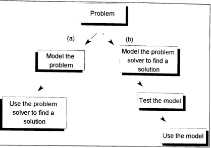
Figure 3.1: A Block diagram showing ( a) the steps followed by the normal system analysis versus (b) Neural Network approach as a problem solver ... 37

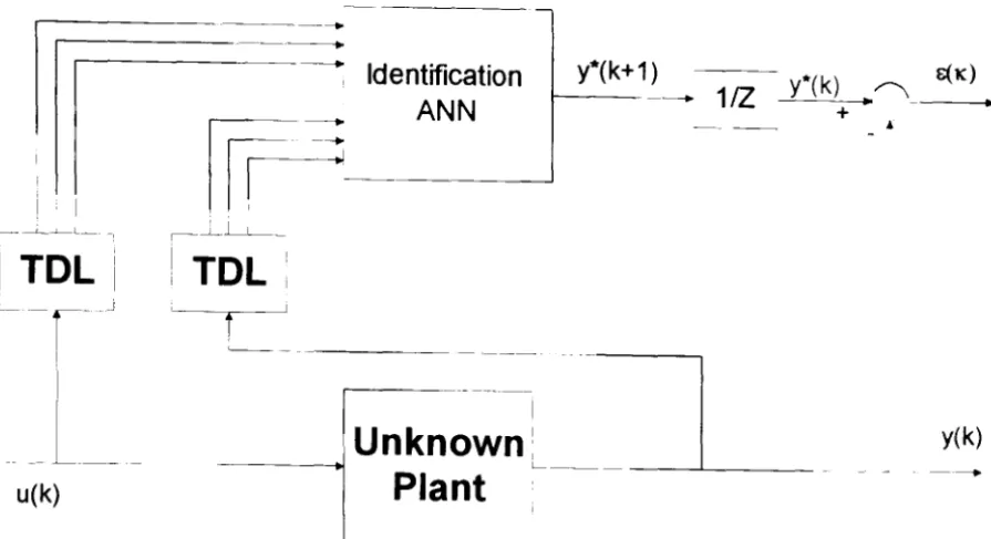
Figure 3.2: System identification using ANNs ... 41

Figure 4.1: A feed forward multi-layer network ... 48

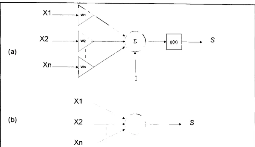
Figure 4.2: (a) Single neuron model, (b) Simplified schematic of single neuron ... 50

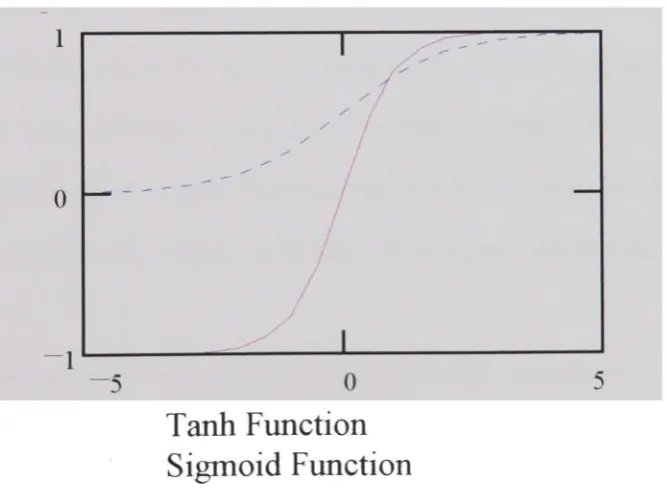
Figure 4.3: The neuron activation function using (a) the tanh function, (b) the sigmoid function ... 51

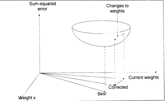
Figure 4.4: An idealized two dimensional error surface ... 54

Figure 4.5: (a) A good fit to noisy data indicated as crosses. (b) Overfitting of the same data: the fit is perfect on the training set, but could be poor on a test set represented by the circle ... 61

Figure 4.6: Architecture of GENE approach ... 66

Figure 4.7: RMS error for output layer ... 70

Figure 4.8: RMS error for Hidden layer ... 70

Figure 4.9: A comparison between the TANH and Sigmoid functions derivatives ... 72

Figure 4.10: Summation & node activation for the TANH function - 1 ... 74

Figure 4. 11: Summation & node activation for the TANH function - 11 ... 74

Figure 4.12: Gradient & error values for the TANH function - I. ... 75

Figure 4. 13: Gradient & error values for the TANH function - II ... 75

Figure 4.14: Summation & node activation for the Sigmoid function - 1 ... 76

Figure 4.15: Summation & node activation for the Sigmoid function - II ... 76

Figure 4.16: Gradient & error values for the Sigmoid function - I ... 76

Figure 4. 1 7: Gradient & error values for the Sigmoid function - II ... 77

Figure 5.1: Test results for modelling MSF plant brine levels (1st and last stage) using BP learning algorithm and 20 hidden neurons ... 89

..

Figure 5.2: Test results for modelling MSF plant with 16 stages using BP learning

algorithm and 20 hidden neurons ... 90 Figure 5.3: Network model simulation results using Tland T2 data after training by

BP algorithm with 4 hidden nodes ... 95 Figure 5.4: Network model simulation results using Tl and T2 data after training by

BP algorithm with 12 hidden nodes ... 96 Figure 5.5: Network model simulation results using Tl and T2 data after training by

BP algorithm with 20 hidden nodes ... 96 Figure 5.6: Network model simulation results using T 1 and T2 data after training by

BP algorithm with 28 hidden nodes ... 97 Figure 5.7: A comparison between BP learning algorithm with different hidden

neurons number for prediction of the first stage level. ... 98 Figure 5.8: Test results for modelling MSF plant with 16 stages using GENE

learning algorithm with 60 neurons for each hidden layer. ... 99 Figure 5.9: Test results for modelling MSF plant with 16 stages using GENE

learning algorithm with 60 neurons for each hidden layer ... 100 Figure 5. 10: Simulation results from ANN using GENE approach, each of the two

hidden layers have 60 neurons ... 101 Figure 5.11: Prediction of the first stage brine level using GENE approach (2 hidden

layers with 75 nodes each) ... 102 Figure 5.12: The block diagram based on cascaded architecture of ANNs and they

are used as an Estimator network (NNE), Controller network (NNC) and

a Mapper network (NNM) ... 105 Figure 5. 13: Block diagram of the proposed neural network for step estimation and

control of MSFD plant ... 108 Figure 5.14: Block diagram of neural network with back-propagation training

algorithm for modelling and set point control function generation for load

variation of MSF unit ... 1 10 Figure 5. 15: Comparison of output error for NNM net during training with different

learning rate at the starting time. Learning is automatically changed with

the learn counts as per table 2 ... 116 Figure 5.16: Output error for NNC net with epoch = 35, with V(t)={VI,V2} as the

input ... 116 Figure 5. 17: Output error for NN C net with epoch = 10, with V (t)= {V I, V2} as the

input ... 116

Figure 5.18: Output error for NNC net with epoch = 10? with V(t)={V1} as the

input ... 117 Figure 5.19: Output error for NNCI net with epoch = 20 ... 11 7 Figure 5.20: Output error for NNCD net with epoch = 20 ... 117 Figure 5.21: Estimated (dark lines) & desired (doted lines) flow values ... 118 Figure 5.22: Estimated (dark lines) & desired (doted lines) temperature values ... 118 Figure 6.1: a simplified nonlinear empirical multi-controller structure for MSF plants .. 133 Figure 6.2: RMS Error values during network learning using the BP (solid)? Gene

with initialized weight 0. 1,0. 1) (dot) and Gene with initialized weight

(-0.05,0.05) (dash) respectively ... 141 Figure 6.3: Error values during network learning for output layer using Gene

approach with initialized weight (-0. 1,0.1) (left) and using Gene approach

with initialized weight (-0.05,0.05) (right) ... 141 Figure 6.4: Error values during network learning for hidden layers using Gene

approach with initialized weight (-0.1,0.1) (left) and using Gene approach

with initialized weight (-0.05,0.05) (right). Solid line for hidden layer # 1 ... 141 Figure 6.5: Error values during network learning using the BP for output (left) and

hidden (right) layers respectively ... 142 Figure 6.6: Test result after first training for cases 3.1,3.2 and 3.3 from left to right.

The solid line and the solid line are for the network prediction and the

corresponding reference respectively. . . .. 142 Figure 6.7: Test result after second training for cases 3.1,3.2 and 3.3 from left to

right. The solid line and the solid line are for the network prediction and

the corresponding reference respectively ... 142 Figure 6.8: Test result after third training for cases 3.1,3.2 and 3.3 from left to right.

The solid line and the solid line are for the network prediction and the

corresponding reference respectively. . . .. 142

Chapter 1

INTRODUCTION

1.1

Introduction

The desalination industry and related control system engineering have now developed in

size and complexity to the point where increasingly sophisticated tools are necessary for

solving the numerous problems that arise in operation, control, planning and design of

these systems. This has seen the introduction of computer technology, the use of

mathematical modelling and programming, control theory and simulation tools. Large

classes of problems however, still continue to elude the above solution methodologies.

These are frequently characterized by imprecision, heuristic decision making, non-linearity,

large size and complexity.

In spite of the significant advances in linear control, the theoretical advances for non-linear

control have been limited. Precise model of process dynamics becomes increasingly

difficult to produce as process complexity increases. Precise modells are required in order

to produce algebraic controller for such systems.

The desalination process is basically an evaporating and condensing process. The heat

required for evaporation can be partly recovered during the condensing phase. MSF

desalination is a type of evaporation with many technical and economic advantages and

can be regarded presently as providing the optimum solution to the problem of sea water

desalting. The basic principles and process description of the MSF desalination process are

CHAPTER 1: _INTRODUCTIOX ..,

Like numerous other models, the model of the MSF is nonlinear in nature. This is mainly

because of the dependence of physical properties of the streams upon temperature,

pressure and salinity. In addition, relations for the heat transfer coefficients also contribute

to the non-linearity of the model. All pervious works for modelling MSF process are based

on the balance equations and the heat transfer equations in the linear form. The physical

property functions that represent a complementary and basic part of the process model are

main contributors to the complexity and non-linearity of the equations. They are the

mathematical correlation expressions describing the thermo-physical properties of water,

steam, and the brine solution. One important requirement of the correlation is their validity

over a wide range of temperatures and concentrations. The evaluation of the overall heat

transfer coefficient for the different stages and the brine heater is another factor of

complexity. It is not possible to completely rely upon the use of mathematical models

based on approximate empirical formula obtained through laboratory work.

Intelligent control attempts to solve difficult or complex problems by admitting process

uncertainty or complexity and relaxing the specification on controlled response, rather

than searching for an exact solution to simplified problems as in classical control. Control

improvement can be achieved by design of a controller whose structure and consequent

outputs in response to external commands are determined by experimental evidence, i.e.,

the observed input/output behavior of the plant, rather than by reference to mathematical

or model-based description of the controller. The controller is then considered as

intelligent controller in which the benefits are through decision making and/or learning

capability. Both approaches can be combined. Dimitris et al (1992) shows that by combining the available prior knowledge of the system with the intelligent controller,

further enhancement can be achieved where the intelligence will be learning and finding

CHAPTER 1: _{INTRODL'CTIOAT}

3

Advanced control techniques are intended to take into account all situations arising in real

plant. AI Gobaisi et al (1991) analyzed the situation in some loops in an MSF plant and

indicated the possibility of improvement by the application of advanced control technique

[2]. The support of artificial intelligent (AI) to the application of advanced control

strategies for the efficient operation of the MSF desalination plants are discussed in

(AIGobaisi et ai, 1994; Rao et ai, 1994) [3], [4]. El-Hawary (1992) discussed possible

application of artificial neural network (ANN) to desalination [5]. The main advantage of

using such an approach is the provision of a general framework to tackle nonlinear control

problems. Moreover, the engineering effort in developing a neural controller is less than

for conventional controller design, at least for nonlinear systems.

In this thesis techniques using intelligent control through the use of ANN for dynamic

modelling. However, model uncertainty, and control prediction are investigated and

applied to the MSF desalination process. Benefits from using such techniques are

discussed with emphasis to the required properties for neurocontrol application. One

technique is based on creating an approximation of the operating conditions in time state

space for specific conditions and network topology. This technique is presented to

demonstrate the capability of Multi-layered Feed forward Network (MFN) for modelling

and control of a MSF desalination plant based on practical examples available from the

process. Comparative simulation results using data from the plant have shown that by

adding more sensory information with proper choice of the learning rate and other learning

parameters, the neurocontroller could generalize for all cases available when it is applied

to the process under consideration. This is a very fast way for estimating controllers set

points once the off-line training is successful. The weak point of ANN with feed forward

configuration is the number of training examples required for generalization and the long

training time. However, an improved technique based on Global Error Node El'alilalioll

CHAPTER 1: _INTRODUCTIOX

propagation learning algorithm is developed. A novel network architecture and learning

algorithm based on the back propagation using the GENE approach is shown to capture

intelligently the dynamics of the system. The main benefit appears when more data are

available for other conditions, the network can be further trained so that the previous and

current learning are working for capturing the function approximation and not just

interpolating the data. It is best suited to on-line approximate calculation. Moreover,

:MFN's with BP learning algorithm are characterized with the static behavior capability,

however, by using this approach considerable improvement is obtained for the

generalization capability of BP for MFN, as well as the technique provides the necessary

dynamic behavior required for the MFN.

1.2

Out line of the thesis

Chapter 2: Overview of Desalination Process

The basic principles and process description of the MSF desalination process are

introduced. Literature review on work done for modelling MSF desalination process

including efforts for dynamic modelling are briefly introduced. Description of the control

system required for MSF desalination process is discussed along with an application of a

supervisory control system for MSF desalination process.

Chapter 3: Intelligent Control

&

Conventional Control System:

An

Overview

Mathematical modelling techniques have been traditionally popular for tasks such as the

study of system behavior, process optimization, process control and the like, but owing to

a variety of reasons like inadequate knowledge about the process, large computational

cost of the attendant simulation etc., alternate strategies might be sometimes called for.

CHAPTER 1: _{INTRODf./CTIOX}

5

Neural networks are essentially multidimensional regression paradigms based on

input-output relationships. They are made to capture the knowledge about the characteristics of

a system through a suitable learning process, so that a tuned network serves as an efficient

tool for simulation studies. The present work attempts to highlight this aspect of neural

networks with a case study conducted on a multistage flash (MSF) desalination plant.

This chapter reviews the literature in applying ANN to the control and modelling problem.

The relationship of intelligent control to traditional control system is briefly reviewed.

Next a comparison with the control system problems solving paradigm is carried out and

lastly a brief overview of intelligent control methodology and application using the

Artificial Neural Networks is discussed.

Chapter 4: Artificial N eural Networks (ANN)

Advances in both learning algorithms and microelectronics have renewed interest in neural

networks across a spectrum of research areas. For control engineering, ANN are attractive

because they have the ability of nonlinear plant modelling, can handle large amount of

sensory information, perform collective processing and learning and offer the potential for

highly parallel computation.

The most important characteristic of ANN is its ability to learn the frequently complex

dynamic behavior of a physical system. Learning is the process where the network

approximates the function mapping from system inputs to outputs, given a set of

observations of its inputs and corresponding outputs. This is done by adjusting the

network internal parameters, to minimize the squared error between the network outputs

and the desired one. One such method is the error back-propagation (BP) algorithm,

which is essentially a first order gradient decent method [6], and is discussed in detail.

CHAPTER 1: _L\TRODCCTION

6

behavior and generalization capability of the ANN. Problems concerning with convergence speed, the number of hidden neurons and the required number of training examples are discussed. A methodology is developed based on global error node evaluation (GENE)

scheme for MFN, that account for generalization and avoiding local minima so that a consistent ANN approach can be developed for dynamic control of MSF. A new method based on GENE approach for MFN is developed. It retains the function approximation requirements for the back propagation (BP) learning algorithm for a nonlinear dynamic behavior. This approach appears to be effective for the input - output modelling of complex process systems and therefore on-line adaptation is possible (when the characteristic of the system is changing or when more test data are available for another operating range). Two problems in BP are addressed, namely, the saturation of the network nodes and the ultimate paralysis of the entire MFN during learning; and the problems of convergence to a local minima. In this approach the architecture is modified by adopting linear activation nodes at the output layer with fixed weights, while the hidden layers (two layers) are having nonlinear activation nodes. The GENE approach is validated using the relationship of the back propagation errors between each layer (output & hidden layers), and the subsequent weight update relation during the whole learning process.

CHAPTER 1: _{INTRODL'CTIOX}

7

can be achieved by keeping the direction of the gradient in the same direction, avoiding the

local minima problem. The internal behavior of the GENE hidden nodes is investigated

and is shown to provide the necessary dynamic/nonlinear behavior that lacks in the

standard BP for MFN.

Chapter 5: Application of Modelling &

Control of MSF Plants by ANN-I

This chapter is devoted to demonstrate the capability of ANNs for modelling and control

of a MSF desalination plant based on a description of practical examples from the

desalination process and results of using ANN s for the simulation, identification,

modelling, and control of MSF desalination plant. This is followed by a brief overview on

the data used for the analysis and the various network structure used for learning. These

include both transients and controlled variables that can be obtained from the various

sensors. Next the ANN controller approach for set - point generation is described and

lastly conclusion is drawn including possible direction of future research.

The approach used in this thesis is described. Data from the plant are used for training and

testing. A Multi layer Feed forward Network (MFN) architecture with the BP learning

algorithm is used and described. Control and modelling capability are investigated by

considering the sample of the system input - output during load change following a time

state space function V(t) with a mapping function N that can be approximated using ANN.

The set point estimation task using the ANN approach is investigated by using two

ANN's; the first one (NNE) has the task of estimating the plant load/status trajectories

during load variation, while the second one (NNC) has the task of producing the necessary

control input based on NNE estimation. Thus the inputs to NNE network are selected as

CHAPTER 1: _{INTRODL'CTlO.Y}

subsequent input to another network. These outputs are the inputs to the control network

(NNe) and the outputs are the manipulated variables (set point to regulatory control).

Chapter 6: Application of Modelling & Control ofMSF Plants by ANN-II

To investigate the response of the control system to external disturbances such that the

plant availability is not disturbed for MSF desalination plant, all main control loops were

observed during imposed disturbances so that the interactions of the desalination process

could be covered. The objective of this chapter is to present a dynamic black box model of

the desalination process. The developed GENE algorithm is applied to data obtained from

MSF desalination plant to identify and model the process behavior due to dynamic

disturbances. The philosophy of applying ANN involve training on part of the scenarios

obtained, and then, using the rest of the scenarios to test and study the network

performance. The study includes the static test (slow variation of the process variables).

The GENE approach is adopted as the learning algorithm, for which it is required to

investigate what dynamic capability could be provided by the feed forward network. The

internal behavior and convergence properties of the algorithm are compared to the

standard back propagation with one hidden layer, and the advantages and disadvantages

are discussed. The results are illustrated using data obtained from AL-T A WEELAH MSF

plant at Abu Dhabi. Satisfactory results are obtained from simulation examples and they

are gIven.

The performance of the network is studied by using dynamic test data from one control

loop in a multi - controller structure for a large-scale process. Next it is discussed what

kind of additional learning method is effective when new dynamic data are available from

CHAPTER 1: INTRODUCTION 9

without affecting the previous learning process. The effective learning method is based on

the Back Propagation (BP) algorithm with a variation or condition in order to: 1) it

approximates an underlying mapping rather than interpolating training samples~ 2) it is

robust against gross error; 3) the rate of convergence is improved since the influence of

incorrect samples is gracefully suppressed. It is important to examine the modelling

capability of different ANN s, to determine what functional, representational and

generalization properties they possess.

Chapter 7: Conclusion

Results for application of the ANN techniques using the GENE approach to predict the

brine levels in the stages of MSF plants are summarized. Further work for the

Chapter 2

_{OVERVIEW OF DESALINATION}

2.1

Introduction

Vitality of water for life growth and lack of natural water sources in some areas of the

world, especially in the Middle East and the Gulf areas, leads to sea water desalination for

fresh water production. Different types of desalination plants are available, with the largest

production capacity being in the conventional multistage flash desalination plants.

Generally the desalination process is by which pure water is separated from a solution of

water and salts. In order to separate the pure water from the concentrated solution we

have to supply some driving force for those separation. The provision of this driving force

results into the energy consumption. Desalination processes can be split in two main

categories:

1) Those where the separation involves a change of phase.

2) Those in which no change of phase is involved.

In the first category, energy is supplied to bring about a phase change between the product

in the vapor form and the concentrated stream in the liquid form. It is important to note

CHAPTER 2: OVERVIEW OF DESAU.\~4 TIO." II

In the second category, the main processes are reverse osmosis and electrodialysis in

which the product and concentrate streams are separated by a physical barrier called a

membrane. The membrane allows the passage of only one material through it and so

desalination is accomplished by the membrane allowing the passage of pure water through

the membrane in case of reverse osmosis and by the passage of the charged ions through

the membrane in the case of electrodialysis.

2.2 MSF Desalination Process

The desalination process in the first category is basically an evaporating and condensing

process. The heat required for evaporation can be partly recovered during the condensing

phase. MSF desalination is a type of evaporation with many technical and economic

advantages and can be regarded presently as providing the optimum solution to the

problem of sea water desalting.

The basic layout consists of a steam source, a water / steam circuit (brine heater) and an

evaporator unit. The plant includes a brine heater and several flash stages divided into two

sections - recovery and reject. The number of stages are determined according to the plant

capacity and performance ratio. Optimum performance ratios are established on a case by

case basis depending of fuel costs, quantity of distillate required, purpose and usage of the

plant.

Steam is fed to the brine heater (to heat sea water) and ejector (to create vacuum). The

circulating water is heated by the absorbed heat from the distillate and passes to the brine

CHAPTER 2: _{OVERVIEW OF DESALJ.\:4 TIOS}

l~

evaporator cells. The evaporator cells have condensers, through which relatively cool

circulating water passes, the condensation takes place thereby producing distillate.

The stages are water sealed from each other to prevent pressure equalization between

stages. Figure 2.1 shows the schematic process diagram of the multistage flash plant, and

is limited to the main elements of the plant which are described in the as following section.

2.2.1

Basic Scheme of MSF Desalination Plant

The cooling water, which is chlorinated sea water from the sea water supply pumps,

enters the plant as the "inlet heat reject flow". It flows through the condenser tubes of the

heat reject stages on which vapor from the flashing brine condenses on the outside of the

condenser tubes. Part of the cooling water heated in this way returns to the sea as heat

reject flow. Only a fraction output of the flow is taken as feed water for the plant and is

called the make-up. This feed is suitably conditioned and for this purpose a dosing unit

and a deaerator are provided. The required make-up is added to the recirculating brine in

the last stage. A combination of brine and make-up is extracted from the last stage of the

evaporator by brine recirculating pump and is then pumped through the condensers of heat

recovery section. The recirculating brine is treated with sodium sulphate to act as an

oxygen scavenger and with antiscale to prevent scale before entering the heat recovery

section. Here the vapor formed by the flashing brine is condensed. When the brine is

recirculated through the heat recovery section condenser tubes, it absorbs the latent heat

of the vapor formed by the flashing brine thereby raising its temperature and finally flows

CHAPTER 2: _{OVERVIEWOF DESAUX4TlOX 13}

steam to the required top brine temperature (TBT). Condensate formed in the brine heater

returns to the condensate header.

From this point the brine flows into the bottom of the first chamber (flash chamber).

Since it is superheated compared to the conditions in the flash chamber it flashes

spontaneously and the brine temperature is lowered in accordance with equilibrium

condition of the stage. The brine at its lower temperature flows through the inter -stage

transfer orifices into the new stage in which the equilibrium temperature is a few degrees

lower. Here, in all the subsequent stages, the flashing process is repeated, so that:

a) The brine cools down in the bottom of the chamber to the accompaniment of

vapor formation.

b) The vapor formed by the flashing brine is condensed on the condenser tubes. The

condensed water called distillate falls into the distillate tray, and

c) The brine in the condensers has its temperature raised. (refer to the "Temperature

Profile" for an MSF desalination plant described below).

Through the flashing which takes place, the salt content of the brine increases stage by

stage and reaches its maximum value in the final heat reject stage.

To prevent buildup of the salt content in the system, it is necessary to tap off a certain

fraction of the brine at some points in the circuit and an equivalent amount of make up is

taken as a feed. This make-up feed water is in addition to the feed water required to

replace the distillate. This is done in the final heat reject stage at the point where the blow

CHAPTER 2: _{OVER VIEW OF DESALI\:-i TJOY}

1~

losses. Since this stage is under vacuum the flow diverted in this way must be extracted

with a pump.

BRINE HEATER

CONDENSATE

EVAPORATOR HEAT RECOVERY SECTlON

ANTI SCALE

DOSING~

Figure 2.1: Schematic diagram ofMSF plant

EVAPORATOR HEAT

REJECTION SECTlON

v

FCV

MAKE \.P

FEED WATER

DISTILLATE

Within the stages the nsmg vapor passes through demisters before reaching the

condensing tubes to prevent the distillate from being contaminated by any entrained sea

water. The demisters usually consists of a closely woven wire mesh. The distillate falls

from the condenser tubes and is collected in wide channels and flows through all the

stages via special inter-stage transfer orifices. In flowing through the stages the distillate

undergoes the same flashing process as the brine flowing underneath. It thereby follows

that in each stage the sum of the distillate and brine flow between the inter -stages is

constant and is equal to the value of the brine flow in the condenser tubes and before entry

into the first flash chamber. Distillate must likewise be withdrawn by a pump from the

final heat reject stage. Vacuum is usually created by connecting the flash chambers and the

non-CHAPTER 2: OVERVIEW OF DES..J,LL\A TlO\" 15

condensing gases, especially all the oxygen and carbon dioxide, which enter with the feed

water and develop in the circuit as a result of thermal decomposition. In general each flash

chamber vents into the next chamber with the non-condensing gases being removed at the

last stage. However, as most of the gases are released in the first few stages, provision is

made such that these are individually vented to the vacuum system.

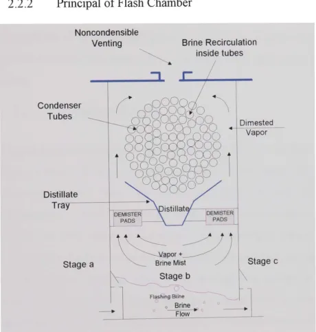
2.2.2

Principal of Flash Chamber

Noncondensible Venting

Condenser Tubes

Distillate Tr y

Stage a

1

Brine Recirculation inside tubes

Stage b

Flash'ing Bone

o Brine Flow

Dimested Vapor

Stage c

Figure 2.2: MSF stage (flash chamber)

The principle of flash chamber is illustrated in figure 2.2. If we take any stage of the

evaporator the water vapor pressure prevailing in the flash chamber will be that

CHAPTER 2: _{OVERVIEW OF DESAU.\~-1 TIOX}

16

the stage b, Pb is lower than that of the preceding stage Pa, but higher than that of the

next stage Pc. It is this pressure difference which draws the brine through the evaporator

stages. The brine enters a stage through the inter-stage brine orifices which are fitted with

a brine gate which may be adjusted from inside the stage. This will enable the optimum

brine level to be established in the stage during plant commissioning. A jump plate is fixed

to the stage floor. This jump plate cause a wave to form thereby increasing the water

depth in front of the brine orifice ensuring the inter-stage brine orifice is fully submerged

and possibility of vapor blow through is eliminated. A splash plate is fixed to the stage

wall above the inter-stage brine orifice to prevent the brine splashing, due to the sudden

flashing

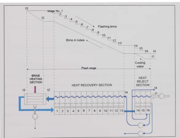
2.2.3

Temperature Profile

A typical temperature diagram for an MSF desalination plant is shown in figure 2.3. The

diagram is divided into three areas corresponding to the heat reject section, heat recovery

section and the brine heater. The cooling water enters the heat reject section at a

temperature of t 1. Within the condenser tubes of the heat reject section its temperature

will rise to t4. This temperature and the brine temperature after flashing in the last stage

are approximately identical, as with equality of these temperatures the vibrations are

minimized. In the condenser tubes of the heat recovery section the brine flow (at

temperature t4) is raised in temperature and on leaving the first stage has reached a

temperature of t2 which also will be the brine heater inlet temperature. In the brine heater

the temperature is increased to the maximum temperature in the circuit t3. This is the Top

Brine Temperature (TBT). From the brine heater the brine flows at a temperature of f 3

into the first stage flash chamber where it is slightly cooled by the simultaneous flashing

CHAPTER 2: _{OVERVIEW OF DESALIXA TIO.\' /7}

temperature than that with which it entered and this change of temperature is

approximately the same for all the stages. In the last stage the flashing brine drops to its

lowest temperature within the circuit 14. This is the Bottom Brine Temperature (BBT).

The total brine temperature range of the plant i.e. the difference between the top brine

temperature 13 and the bottom brine temperature 14 is called the "working range" or the

"flashing range". The temperature of the distillate is lower than that of the flashing brine

flowing beneath it by approximately 1 to 1.5 oC, i.e. by the amount of the boiling point

elevation of the flashing brine and of various other temperature losses in the stage e.g.

non-equilibrium, non-condensing gases, demister and bundle losses.

t3

t2

BRINE I

I HEATING I

SECTION I I

t3 :

I

Flashing brine

Brine in tubes

HEAT RECOVERY SECTION

6 t4

I I t1

I

I Cooling I water

I HEAT I I REJECT I

I SECTION I I I t4

"-__ --.

1

CHAPTER 2: _{OVERVIEW OF DESAUA:4TJO.Y}

ilJ

4. Feed (makeup) flow rate/anti scale flow ratio

5. Brine blow down flow

Detailed description of the process control system is as follows:

1. The sea water flow rate to reject section is regulated so that the sea water from reject section temperature is equal to the temperature of the brine in the first stage which is

the temperature of the brine recirculation at the pump discharge or entering the heat

recovery section through the condenser to keep the heat balanced in the process. Sea

water flows to the heat reject section depends on seasonal conditions (summer or

winter) and is maintained by actuating the sea water discharge valve or by varying the

speed of the sea water supply pump employing PI controller.

2. The brine recirculation flow is regulated to increase / decrease the production as it will

increase/decrease the brine flashing rate. It will affect the quantity of brine that remains

inside each stage. This must be done properly so that no disturbance occur in the levels

of the brine in the different stages. The level in each stage should not be so high so that

the carry over is encountered, which is the contamination of distillate product which

result in higher salt content of the distillate than the required design level. At the same

time the level should not be so low that will lead to blow through flow in the

inter-stage. To maintain the brine flow rate, signals from electromagnetic flow transmitters

are used to actuate the respective control valve. The objective is to maintain the brine

recirculation and distillate flow rates at the required value in response to seasonal

(summer, versus winter), and high temperature chemicals conditions affecting the flo\v

CHAPTER 2: _{OVERVIEWOF DESAUHATIOX}

:0

3. The feed (makeup) flow rate is regulated so that the salinity of the recycled brine is controlled at a constant optimum concentration, this is achieved by a ratio control with the flow rate of the distillate drawn from the plant.

4. The control of distillate product flow is by regulating the Top brine temperature and

the brine recirculation flow in reasonable sequences and at a rate of change that does

not affect the equilibrium of the process. This rate is usually determined at site. The

required brine temperature in order to produce a certain distillate product is regulated

by variation of the steam temperature and flow rate to the brine heater. The steam

temperature variation is achieved by variation of the de-superheating water flow. PID

control is employed in the temperature controller. The steam pressure in the brine

water is normally used as an auxiliary variable in the cascade control mode.

5. Brine level in the last stage chamber of the evaporator which is directly related to the

levels in the preceding stages, is maintained at a predetermined set point. The PI level

controller actuates the brine blow down valve. In the case of a brine blow down pump

equipped with variable speed control, level control is done through speed change. For

the system material balance it is required to keep the brine blow down flow rate equal

to the difference between the makeup flow rate and the distillate output.

Additional loops such as the chemical injection loop, and sea water make up flow loop

may be integrated in the overall control system. Further improvements are obtained when

additional loops are added such as blow down flow, sea water recirculation, and heat

reject section inlet temperature.

CHAPTER 2: _{OVERVIEW OF DESAU~\:J. TIO;\' ]}}

Control of MSF desalination plants is generally based on conventional PID controller for

TB T and only PI for the rest of the variables. However a derivative control function may

be added if a fine control is desired. The controllers function fairly well when set properly

at or near the best desired and calibrated set points. When a disturbance takes place,

conventional controllers do not perform satisfactorily because the controller parameters

settings do not correspond to the disturbance encountered.

MSF desalination plants with considerable amounts of mass and energy require novel

types of high performance controllers that are almost always digitally based and perform

control functions based on many available modern control algorithms.

Adaptive control (or self tuning control) offers one solution to the manual tuning of PID

controllers, by attempting to maintain good robustness even if unpredictable changes

occur in the process, sensors, and probably due to damage to the controller itself The

basic idea is to combine an on line parameter estimation procedure with some control

system design technique to produce a control law with a self tuning capability. These

controllers are capable of tuning themselves to optimal settings and returning whenever

the process dynamics / behavior changes. The application of high performance controllers

can result in a stable, efficient, smooth operating plant with extended life span. Adaptive

control is successful only if a model exists with sufficiently accurate parameters. Model

accuracy can be improved using artificial intelligence [3], [4].

For MSF desalination, control system design requires a knowledge of the inherent plant

dynamic behavior, the really crucial flow-related control parameters are not those which

are directly observable (such as temperature, flow, and pressure). Instead, they are the

CHAPTER 2: _{OVERVlEWOF DESALL\~-4TIOX} ..,.,

tube bundles, non-equilibrium losses in flashing of brine, and the stability of tray brine

levels and inter-stage flows. Measurement of these phenomena must be derived from the

direct measurements often requiring considerable accuracy. Proper modelling to

understand the plant dynamic behavior is required and it would be great if the brine levels

could be estimated accurately.

Like other processes, other modelling difficulties appears from the requirement for the

inclusion of complex process characteristics such as time delays, disturbances, unmeasured

variables, time-varying parameters, nonlinearities and multivariables interactions. While

microcomputer based controllers are adequate hardware that is theoretically adequate to

overcome these problems, the challenge is to find the appropriate software to direct the

hardware. Artificial neural networks provide an innovative new paradigm that is

beginning to be applied to these areas with excellent results.

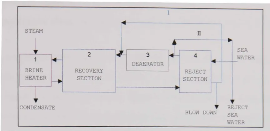
2.4

The Dilemma ofMSF Process Modelling

In general, the MSF process, as shown in figure 2.5, contains two recycle loops I, II. In

the major recycle loop, part of the brine is recirculated to merge with the make-up flow.

this combined stream, flowing counter currently to the flashing brine, is heated in the

recovery section until it enters the brine heater. The second loop results by recycling part

of the cooling water from the reject section to maintain constant cooling water

temperature at the entry of the reject section (during the winter season).

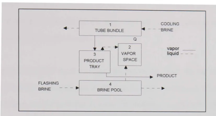
The recovery and reject sections contain several stages. Each stage can be considered

containing four compartments as shown in figure 2.6, namely, brine pool, product tray,

vapor space and tube bundle; among these compartments the vapor and liquid flows are

CHAPTER 2: _{OVERf/1EWOF DESALI.\"ATlO.\"}

I

~

--STEAM _II

~

.4

,

1

4

1 ~ WATER

DEAERATOR I

BRINE RECOVERY I REJECT

HEATER

~ SECTION J SECTION _""T

~

,

.

CONDENSATE

•

BLOW DOWN _SEA WATER

Figure 2.5: MSF process block diagram

Each fluid stream communicating with the individual stage has four attributes: Flow rate.

temperature, pressure, and salt concentration, which can be considered as independent

variables. For a detailed modelling the conservation of mass and energy for each stage

must be satisfied, which are influenced by other stages. The model present a large scale

problem where several hundreds of nonlinear equations must be solved. Various

approaches were employed for solving such a model of nonlinear equations. One approach

is based on the solution of these equations by stage to stage calculations, which is

characterized by instability and low rate of conversions (e.g.: Beamer et al [7] used a

stage to stage model with calculations being started at the hot end of the plant in an

optimization study. A similar approach was used by Barba et al [8] where initial guess,

provided by a simplified model which calculates the main dependent variables, were fed to

the main mode1.). Another approach is to develop a rigorous method for solving the

detailed steady state model which is based on the decomposition of the large set of

equations into a smaller subsets followed by iterative sequential solution of these subsets.

Rautenbach and Buche} [9], Orner [10] and Medani et al [11] followed a sequential

approach with certain optimization program to minimize the stage wise fashion

calculations starting at the hot end of the plant. Helal et al [12] linearized the governing

CHAPTER 2: _{OVERI7EWOF DESAUNATIOX}

tridiagonal matrix (TDM) technique originally proposed by Amundson and Pontinin [13]

and was improved by Wang and Hanke [14] and was employed by Husain [15], [16].

To obtain a rigorous model for the MSF desalination process, a total mass, component

and enthalpy balance can be written for each of the four compartment divisions of a stage

shown in figure 2-6, plus heat transfer equation between the tube bundle and a vapor

space. In addition, one has to consider that the evaporation process occurring in the brine

pool is a constant enthalpy process. With time derivatives included, such a generalized

model serves as dynamic model; when these derivatives are put equal to zero it represents

steady-state condition [17]. This model has to be supported by accurate correlations for

brine densities, boiling temperatures, brine and vapor enthalpies, and heat transfer

coefficients. These parameters/coefficients which in the two-phase section is different from

the parameters for one-phase section. They depend on the fraction of vapor, fluid velocity

and the difference between pressure in the stage and the previous stage. In addition, there

are temperature losses between the brine pool and the vapor space due to boiling point

elevations, non-equilibration in the pool and pressure losses in the demisters and across

the tube bundle, which must all be accounted in a representative model. Furthermore,

there are uncertainties such as the fraction of the total evaporation which takes place from

the product tray is not separately known. In a solvable analytical model along the above

lines, simplifications lead to inaccuracies for which the main sources are the following :

• Heat transfer coefficients: the theoretical values differing 10% or more from those

calculated from the actual plant operating data [7] may be due to the presence of non

condensable gases. In addition, heat transfer rates decrease with time due to fouling.

For on-line simulation, periodical measurements and calculations are necessary.

• During flashing if the thermal equilibrium is reached, then the temperature of the brine

CHAPTER 2: _{OVER VIEW OF DESALl.\~-1 TIOS}

elevation. Normally, the equilibrium is not reached, therefore, there is an additional

temperature loss that has to be accounted for in order to properly evaluate the vapor

temperature.

1 COOLING

..

-TUBE BUNDLE - - -SRINE

1.

-

...

2 _{vapor _ _}

3 VAPOR liquid -PRODUCT SPACE

TRAY

•

I I _PRODUCT

I ...

FLASHING

1

~---

~

BRINE - -

-I

Figure 2.6: Representation of a single stage of the MSF plant

As regard the overall enthalpy balances, two approaches are possible, a local and a global

approach. The balance is made with respect to terminal streams in each stage for the local

approach. Whereas in the global approach, heat input to either recovery or reject sections

is taken into account in making an enthalpy balance for each individual stage [8].

2.5

Supervisory Control System for MSF Desalination Process

One of the primary concern is to maintain the water production under all circumstances.

MSF process startup requires the preparation of the vacuum into the stages and this

requires some time and effort from the operator to create the vacuum required for the

operation. For this plant shut down due to any disturbance is required to be avoided.

Additionally load variation is frequently required in large MSF units. Hence a smooth,

reliable and efficient control is required by the operator through the interface station for

CHAPTER 2: _OVERT7EHl _{OF DESALIX4TIOX}

l6

controlling the heat input to the brine heater by decreasing / increasing the TBT controller

set point in predetermined steps. For each step of the TBT change, the brine recirculation

flow rate is also suitably changes in sequence. These steps are repeated until the required

distillate product is achieved. The rate of change of the above parameters, determined by

the amount of change in the set points in each step and the time between two successive

steps, is judged by the operator on site.

Manual control of the MSF plant is a hard task for the operator and the dynamic model,

considering the previously mentioned conditions, is quite complicated. Therefore, efforts

have been taken to use the computer to assist the operator. A computer supervisory load

variation control can be adopted and this has been realized at various locations in the

Arabic Gulf such as Abu Dhabi and Oman [18], [19]. However, a dynamic model has not

been used.

The values of the set points are calculated according to the followings:

• The brine recirculation flow rate is calculated using the operating curves as function of

the product distillate flow rate and the cooling water temperature (reject inlet).

• The cooling water flow rate is function of the cooling water temperature (reject inlet)

• The TB T is calculated using the heat and mass balance of the evaporator and changes

according with the changes in the fouling factor and in the sea water temperature.

• The steam temperature to the brine heater inlet is calculated according to the TB T .

The calculation is performed in order to limit the degree of superheating of the steam

at high load, and according to the maximum de-superheating water flow rate at low