Teach and repeat path following for an autonomous underwater vehicle

Teach-and-repeat path following for an autonomous

underwater vehicle

Peter King Australian Maritime College

University of Tasmania Australia pdking@utas.edu.au

Andrew Vardy

Department of Computer Science

Department of Electrical and Computer Engineering Memorial University of Newfoundland

Canada av@mun.ca

Alexander L. Forrest Australian Maritime College

University of Tasmania

Department of Civil and Environmental Engineering University of California, Davis

USA

alforrest@ucdavis.edu

Abstract

either to return to the start location, or to repeat the route. Utilizing unique assumptions about the sonar image generation process, this system exhibits robust image matching ca-pabilities, providing observations to a discrete Bayesian filter which maintains an estimate of progress along the path. Image matching also provides an estimate of offset from the path, allowing the AUV to correct its heading and effectively close the gap.

Over a series of field trials, this system demonstrated online control of an AUV in the ocean environment of Holyrood Arm, Newfoundland and Labrador, Canada. The system was implemented on an International Submarine Engineering Ltd. Explorer AUV and performed multiple path completions over both a 1kmand 5kmtrack. These trials illustrated an AUV operating in a fully autonomous mode, in which navigation was driven solely by sensor feedback and adaptive control. Path following performance was as desired, with the AUV maintaining close offset to the path.

1

Introduction

Autonomous Underwater Vehicles (AUVs) are free swimming robots that traverse some of the most remote and dynamic environments on Earth. These environments include beneath floating ice shelves (Jenkins et al., 2010) and under moving sea ice (Kaminski et al., 2010). In these scenarios, AUVs are required to traverse long distances away from a known safe launch-and-recover site. Where the environment is unknown and diverse, a path the AUV has taken previously may be one of, or the only, safe passage to and from a particular site. In these instances, it is imperative that an AUV has the ability to retrace its steps and follow a path it has traversed before.

Geophysical referencing allows an AUV to position itself using sensory feedback. If a reference map is provided in advance of a mission, localization occurs by comparing local measurements against the map to limit the probable locations. When combined with knowledge of the vehicle motion, an estimate of position can be obtained; this is generally referred to as Terrain Relative Navigation (TRN). Examples of TRN adapted for underwater vehicles are presented in (Claus and Bachmayer, 2015; Rock et al., 2014; Meduna et al., 2008), with a general overview of systems provided by (Chen et al., 2015). Another approach is to simultaneously generate a map of the area and localize to it, known as Simultaneous Localization and Mapping (SLAM). This is an active field of study and many example systems exist (Paull et al., 2014; Mahon et al., 2008; Tena Ruiz et al., 2004).

An alternate geophysical approach is teach-and-repeat (TR) path following, which does not require the estimation of position in the global reference frame, but only with respect to previously collected data. This lack of positioning requirement allows for a less complex system than SLAM. TR enables an autonomous vehicle to re-follow a path by relating its current sensory input to a stored sequence of sensory input from a previous traversal. TR localizes the agent relative only to the path, and does not rely on a global localization of either the robot or locations along the path (Matsumoto et al., 2000; Furgale and Barfoot, 2010; Nguyen et al., 2016). For long-range exploration missions, TR allows an AUV to venture into an unexplored area and return along the same path, regardless of its accumulated global position error.

Presented here is an adaption of TR for an AUV that builds upon similar work in the terrestrial robotics world, with adaptations to an underwater vehicle. The contribution of this work is the successful imple-mentation of Teach and Repeat path following on an Autonomous Underwater Vehicle utilizing sonar as the primary imaging sensor. This implementation has been demonstrated with multiple successful field demon-strations of fully-autonomous path following in a true ocean environment over paths up to 5km in length, with the vehicle under fully self-determined adaptive mission control. The success of this system relies on improvements made to image registration techniques, capitalizing on the unique aspects of the sonar imaging used in this work.

2

Methodology

For a geophysical navigation system, how the environment is perceived is critical to its ability to localize and determine any required corrective actions. The primary development in adapting teach-and-repeat (TR) to an underwater vehicle was the use of images derived from available sonar data. This section provides an overview of techniques used for image generation and matching.

2.1 Target Platform

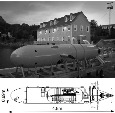
Development of this system was for Memorial University of Newfoundland’s (MUN) Explorer AUV, shown in Figure 1. The MUN Explorer is a 4.5mlong, 3000m depth rated vehicle manufactured by International Submarine Engineering (ISE) (ISE, 2016; Lewis et al., 2016). This survey class AUV can traverse distances over 100kmand navigates using a true-North sensing fibre optic gyroscope and a Doppler Velocity Log (DVL), capable of providing velocity relative to the seabed at altitudes less than 200m. Additional operational specifications are given in Table 1.

Figure 1: Memorial University of Newfoundland’s Explorer AUV.

2.2 Vehicle Integration

Table 1: System Specification of Memorial University’s Explorer AUV

System Components Specification

Navigation DGPS, iXBlue Fibre Optic INS, RDI Doppler Velocity Log (300kHz)

Positional accuracy to 0.1% of dis-tance traveled when submerged and relative seafloor velocity provided by DVL. Heading accuracy to 0.01◦ Payload Edgetech 2200m, SeaBird CTD 400kHz sidescan sonar. 200m

maxi-mum range per side, 75m for this work at 7m altitude. Processed resolution to 0.2m at 1.5m/s survey speed.

Processing Payload Computer 2.1 GHz Intel i7, 4GB RAM, 128GB SSD

navigation estimate. This was hosted on a dedicated payload computer connected to both the sonar and AUV control system though Ethernet. The second is a control interface to allow incoming requests from the payload computer to affect the movement of the AUV. The manufacturer, ISE, provided a set of short messages which would allow the processing computer to request control, provide a new target to navigate toward, and relinquish control.

At the start of the workflow the AUV is given a mission script to follow, essentially a series of waypoints. This phase, referred to as the Discovery phase, is merely an intermediate step between the teach and repeat phases. Upon the TR system making a match and achieving a belief in its location above a threshold,

min belief localize, a control request is sent to interrupt the current mission and await location targets, this is known as the Repeat phase. At any time the TR system can relinquish control and the AUV will return to the last executed step in the previously interrupted mission script. Figure 2 illustrates this workflow. It should be noted that in practice, returning to the previous executed mission may not be advisable, but suited the test scenario.

2.3 Image generation

For underwater vehicles, sonar is the primary means for sensory feedback from the environment, given the attenuation of optics in water (Al-Shamma’a et al., 2004). This work focuses specifically on sidescan sonar, for the following reasons: it is commonly found on survey class AUVs; it provides a value of reflected intensity that lends itself to the construction of a grayscale image; and, it has an operational range that allows coverage over a large area whilst operating the AUV at safe distances from the seafloor.

Figure 2: Flowchart of AUV interaction from Discovery to Repeat phases. Flow is from top to bottom, with final decision on the current mode based on believe being either above,>, or below,<, a threshold.

in the along track dimension and wide across track. This is illustrated in Figure 3. Reflected intensity decreases as the beam travels away from the AUV, increases when encountering a strong reflector, such as the illustrated rock, and may reduce to nil in the shadow zone behind obstructions, as can be seen on the side of the rock furthest from the AUV. The intensity of the measured reflected signal is dictated by the reflectivity of the seabed material, angle of incidence to the bottom or objects, occlusion, and the normal loss of sound intensity as it moves away from the source (Pinto et al., 2009). In addition there will be an area of poor coverage directly below the AUV, known as the Nadir. The sonar used in this work had a maximum operating range of 75mfrom each side of the AUV, for a total coverage width of 150mat a fixed altitude of 7m.

The AUV measures its true heading and speed relative to the seabed to construct a two-dimensional projec-tion of the sonar intensity by georeferencing sequential sonar pings onto a common North-up image grid of fixed resolution. These images assume a localized flat bottom with intensities corrected for attenuation such that relative intensity variations in the image are related to artifacts of the seafloor and not to propagation of the sound energy. Figure 4 provides examples of generated images. A more detailed description of the image generation process used in this work is provided in (King et al., 2012). A distinguishing feature of sonar images is the blank nadir region, which is masked out in this work to ignore poor image quality directly below the vehicle.

Figure 3: Top: Overhead view showing coverage area of a single sonar ping, the ping encounters a rock, which acts as a strong reflector. Middle: Rear view showing the occlusion of the sonar beam by the rock. Bottom: Relative intensity over the horizontal dimension. Intensity decreases as we move away from the AUV, becomes stronger as it reflects off the rock, then turns to shadow in the region occulded by the rock.

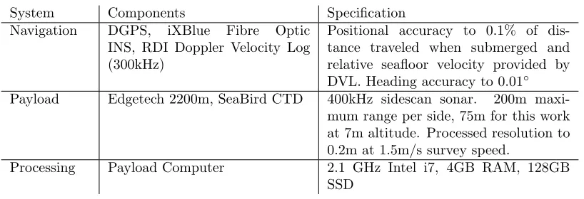
Figure 4: Example sonar images. The boundaries of the sonar data (including the Nadir) are masked to ignore any deformations, hence the black regions. Left: A flat sandy area showing a patch of gravel. Right: A regions with visible scour marks.

2.4 Image matching

orientation differs. Image matching techniques utilized in this work rely on feature extraction and matching and include SIFT (Lowe, 2004), SURF (Bay et al., 2008) and FREAK (Alahi et al., 2012), with implementa-tions taken from the Open Source Computer Vision Library (OpenCV) (Itseez, 2015). Preliminary work on the selection and characterization of the chosen feature matching techniques as they relate to sonar images are described further in (King et al., 2013; Vandrish et al., 2011).

At its core, feature extraction is the process of locating areas of interest in an image, referred to as keypoints. These keypoints are expected to be consistently discernible from repeated views of the same image subject. Keypoints are described by the size of their included pixel neighborhood, as well as an orientation, derived by the dominant gradient component of the feature. Figure 5 illustrates a single sonar image and the detected set of keypoints drawn with relative size and direction indicators.

Image matching is the determination of the likelihood that two images represent an overlapping view of the seabed. If we assume that keypoints are fixed artifacts of a particular area of the seabed then two overlapping views may contain the same keypoints. Thus, if two images are compared based on keypoints we can infer a likelihood they represent a common view of an area of seabed.

2.4.1 Match filtering

The image match filtering process described here is a key contribution of this work. Its effectiveness stems from the unique characteristics of images produced from sonar data. The process is to compare the set of keypoints in one image to those of another image to form a set of candidate match pairs. In this work, an exhaustive matcher was used in which each keypoint in the first set is compared against all keypoints in the second set to select the closest match. This initial brute force pairing of best matches produces a large pool of pairs containing many likely false matches. The goal of the filtering process is to reduce this set to those pairs that are likely to be true matches.

To extract the true matches from all possible matches, we avail of two invariants:

1. given the AUV’s ability to directly measure its true heading, the generated images share a common North-up orientation; and,

2. given the AUV’s ability to measure its height above the seafloor the generated images are projected onto a common flat plane, thus they share the same scale.

Therefore, common keypoints across images should be similar in both size and orientation, quite different than what is experienced in optical images of natural terrestrial scenes. These invariants hold up in areas of relatively flat terrain but have been untested in areas with a sloping or more dynamic terrain.

The initial set of matched pairs are subjected to a filtering stage to disregard mis-matched keypoint pairs. Allowing for some error in the AUV’s orientation and ability to scale generated images, keypoint matches that differ in size or orientation beyond some nominal threshold are considered non-matches, and are discarded, Algorithm 1 includes the filtering steps. This threshold is a tuned parameter and, in these results, was set based on prior offline testing, described further in (King et al., 2012).

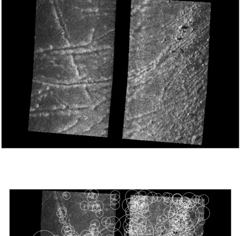
resulting geometric transformation between them must be solely translation, with negligible rotation or scaling. For a given pair of images with multiple feature matches, true-matches will represent a common feature translated from one image to another by a common offset. Conversely the feature offset in a false-match will be unpredictably distributed.

Figure 6 illustrates this process, where two views, indicated by the dashed boxes, overlap over a set of features. The resultant images have the features located in differing locations, based on the orientation of the view. When compared we can see how the features must translate from one image to another and that good feature matches have offsets consistent in both direction and displacement.

2.4.2 Match consensus

To determine a consensus within the raw matches, given our already filtered set of matches and constraints on orientation, it is possible to employ a brute-force consensus algorithm which determines the largest possible inlier set of matches satisfying the invariant. Again the ability to rely on a common scale and orientation greatly improves match performance. This differs from the more common use of methods based on the Random Sample Consensus algorithm (RANSAC), which provide a suitable consensus within a group, but not necessarily the largest or optimal consensus (Fischler and Bolles, 1981).

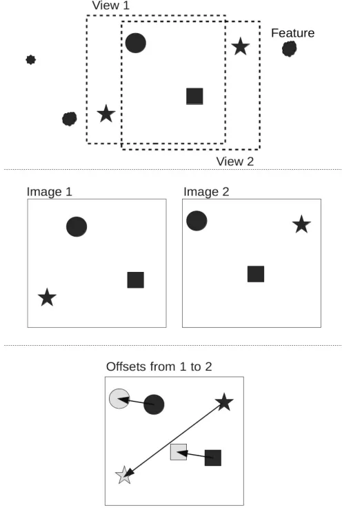
This complete matching algorithm, provided in Algorithm 1, includes the steps for determining consensus. Every possible group of matched pairs, with similar orientation and lateral displacement within a specified threshold, is considered. The largest of these groups determines the estimate of geometric translation, with match pairs outside this group rejected as outliers. Figure 7 illustrates the steps in image match determination for both the matching and non-matching cases. Should no inlier group exist, or is smaller than a set threshold, no match is assumed to have occurred. In the event of two inlier groups having equal size, an event not seen in all testing to date, the system would only consider the first largest set encountered.

Figure 7: Top: sonar images with raw keypoint matches. Middle: remaining matches after filtering on size and orientation. Bottom: only matches from the largest consensus group.

Algorithm 1Matching algorithm

1: function_Match(refImageSet, image)

2: for allref Img inref ImageSetdo

3: matches←imageMatcher(image,ref Image) .result of the image matching

4: goodM atches←empty

5: for allminmatches do . Filter keypoint matches

6: if abs(m.train.size−m.query.size)< sizeT hreshold then

7: if abs(m.train.angle−m.query.angle)< angleT hresholdthen

8: _Append(goodM atches,m)

9: end if

10: end if

11: end for

12: for allmi ingoodM atches do . Determine consensus for inlier keypoint matches

13: inliersi←empty

14: projection←(mi.train.xy−mi.query.xy)

15: for allmj ingoodM atchesdo

16: if mi! =mj then

17: error←mj.train.xy−mj.query.xy−projection

18: if error < minReprojectionthen

19: Append(inliersi,mj)

20: end if

21: end if

22: end for

23: end for

24: _Append(inlier sets,inliersi)

25: end for

26: returnGetLargest(inlier sets)

27: end function

3

Teach-and-repeat path following

Teach-and-repeat path following allows a vehicle to navigate along a previously traversed path. The path, as described by Matsumoto et al., may be a sequence of view images, each with information describing its relation to the next image in the sequence. During training, images are added if they represent a significant change in view. During the repeat phase, image matching is employed to compare the current view against the estimated subsequent training image. If the subsequent image has a higher correspondence, the estimated location along the route is incremented. Image matching is used to determine the correspondence between images and the azimuthal offset between them. The offset is used to direct the robot toward the center of the path, allowing correction of horizontal offsets from the prescribed route (Matsumoto et al., 1996).

An example of this type of system presented by Furgale et al. models the path as a topologically connected set of sub-maps, where only the sub-maps are described as locally euclidean. Localization is based on a combination of feature detection and knowledge of the robot’s motion. Several trials of the system are described, with the longest a 32km route over rough outdoor terrain (Furgale and Barfoot, 2010). The motivation of their work is to support extra-planetary exploration by robots, a field not unlike that of exploratory AUVs.

In this work, the path is constructed by continuously generating sonar images, consisting of a fixed number of individual pings, of the seafloor and storing them as a connected series of images, with information of how each subsequent view connects to the next; we refer to this series of views as the reference path, and each individual view a node. As in (Furgale and Barfoot, 2010), the constraints are that the images are locally consistent with reasonable transformations between them. In the context of this work the transformation is minimal as each view connects to the previous such that they are essentially seamless. Unlike the work of (Matsumoto et al., 2000), every completed image is added to the path, given the nature of the sonar collection they are distinct. The AUV’s internal navigation system provides the node-to-node relative positioning.

Localization along the reference path is one-dimensional, as the AUV only needs to know at which node it is most likely at. The arrangement of each view is topological, but not globally topographic, such as in (Matsumoto et al., 2000; Matsumoto et al., 1996), referred to as Visual Sequenced Route Representation (VSSR). We are simply concerned with the relative relation of views to each other and not the precise placement relative to a coordinate system, Figure 8 illustrates this concept.

Figure 8: Representation of views as locations along a path: Left: sonar images as there are collected by the AUV; Middle: the vector of nodes, where location is a single dimension index; Right: Data stored with each node, including ID of previous and next node, and average heading along the node.

actions may be determined to maintain its track along the path to completion. The likelihood value provided by the image matching gives a quantitative measure of which nodes the AUVs current view matches. But, this is insufficient as there is the possibility that: a) the AUV matches to multiple locations, b) the AUV makes no match and thus gains no insight into its location, or c) the AUV matches to a single incorrect location.

To maintain a robust estimate of the AUV’s location along the route a discrete probability filter, or Markov Localization filter, is employed, similar to the along-route localization employed in (Zhang and Kleeman, 2009). The Markov localization filter maintains an array of probabilities, representing each node in the path, where the probability is the belief that the AUV is at that node. This array represents the probability distribution of the AUVs location along the route. At any given time, the array location of the distribution peak is taken as the current location estimate. If this peak is above a specified threshold, the vehicle is considered localized at the corresponding path node.

This distribution is updated in two steps: a prediction step, accounting for the AUV’s motion; and, an observation step, accounting for the current sensor view. This filter suits this problem due to its inherent discrete nature and the condition that the AUV may face phases of global uncertainty due to a difficult data association problem where matches yield multiple hypothesis, as stated in (Thrun et al., 2005).

a particular node is based on the sum of probabilities that the AUV has moved to this node from all possible previous nodes, stated as:

p(ni,t) =X j

p(ni,t|ut, nj,t−1)p(nj,t−1)

= p(ut=stay)p(ni=nj) +p(ut=move)p(ni−1=nj)

(1)

Wherep(ni,t) is the estimated probability of being at nodeiat time stept. p(ni,t|ut, nj,t−1) is the probability

of moving to node i from nodej, given some action u. In this system there are only two possibilities of arriving at ni: already being atni in the previous time step and not moving, and, moving to ni from the prior node in the sequence, ni−1. For the linear type paths attempted in this work and the fine control of

the AUV, we assume the AUV can only remain at a node or move forward. For this work, we repeat the path at the same speed as was taught, thus we maintain a high probability of reaching the next node in one update cycle. For completeness the probability of moving follows:

p(u=stay) = 1− p(u=move) (2)

The likelihood of an observation at a node results from the image matching and the current localisation estimate outcome of the prediction step. As stated in the previous section, this likelihood, or measurement value, relates to the consensus of feature match pairs:

p(ni,t) =p(zt|ni,t)p(ni,t) =

S+Pci Nci

p(ni,t)

(3)

matches to all other nodes. Thus the likelihood measure grows as there are more good matches, but is diluted as there are more total matches in other nodes.

The Markov filter algorithm is given in Algorithm 2.

Algorithm 2Markov Localization

1: function_localize(p(n), c(n))

2: foriinp(n), c(n)do

3: p(ni)←p(u=stay)p(ni−1) +p(u=move)p(ni) .prediction

4: p(ni)←S+ c(ni)

P_c(n)

p(ni) . observation

5: end for

6: p(n)← Pp(_pn₍)_n)

7: returnp(n)

8: end function

From each filtered match, an offset between images is provided, in pixels, for both the x and y axis. The mean offset is then calculated for all remaining matches and converted to a physical offset in both the North and East axis, based on the image resolution:

of f seteast=of f setx×grid resolution

of f setnorth=of f sety×grid resolution

(4)

wheregrid resolutionis expressed as meters per pixel. The translation is the distance between the AUV’s current position and the location it was when the reference view was captured. To maintain a consistent re-tracing of the path the offset, with respect to the centerline of the path, should be reduced.

When a successful localization is made a vector addition is performed between the offset vector and the path vector connecting the current estimated node to the next. There is no separation between each view - the end point of one image is adjacent to the start point of the next image in the reference path - thus, when localized, the AUV is assumed to be offset from the end point of the current estimated node, or at the start of the next node in the path. If we add the offset vector to the vector across the next node in the series, we will perform an action to both close the offset and to traverse the path.

Figure 9: Top: AUV following path using the stored node-to-node vectors, but with an offset. Bottom: Corrective vector from image matching added to path vector so that the AUV will reduce its offset.

Figure 10 illustrates the processing of a new sonar file and the exchange of data between the major compo-nents. Figure 11 expands the calculation of a new navigation target.

Figure 11: Flowchart of navigation determination

4

Field Trials

Tests of the complete teach-and-repeat system were conducted in May, 2013 and November, 2014, in Holyrood Arm, Newfoundland and Labrador, Canada. This is a sheltered 5km inlet with water depths ranging from 20m−80m. Prior surveys had been conducted in this area allowing empirical configuration of the sidescan parameters based on repeated processing of the previously collected sonar data.

Tests were performed on two predefined reference paths: a short path for initial testing in 2013, repeated in 2014; and, a longer path only attempted in 2014. In each scenario the reference mission plan was traversed in teach mode and the resulting reference path then utilized for multiple repeat attempts. Figure 12 show the reference paths used in testing. On each repeat attempt the AUV conducted a prescribed mission which guaranteed it to both cross the reference path, and then pass alongside, whilst generating sonar images, in an attempt to make an initial match and localization to the reference set — the discovery phase. If a strong match was made to provide the initial localization, the TR system requested an interrupt to the ongoing mission, entered the repeat phase and attempted to follow the reference path to completion. The trials provided an opportunity to test all aspects of the TR system: image matching, localization, navigation and autonomous AUV control.

Figure 12: Reference paths for field trials shown in black. Shorter path used in 2013 trials and repeated in 2014. Longer path used in 2014 trials only. Location is Holyrood Arm, Newfoundland and Labrador, Canada.

approach was thought to be the most difficult and thus the worse case scenario.

In the following field season, a repeat of the shorter path was conducted to ensure continued development of the system and the vehicle had not affected the performance of the TR system. This development included bug fixes, refactoring for improved efficiency and the inclusion of additional feature detection algorithms. In these tests the same reference path route as the previous year was utilized, but with a shortened North-South line due to deployed fishing gear, giving 20 individual image views. A longer route was also used to further show the performance and utility of the system for extended operations. In this test a South to North route following the Eastern coastline was selected. This reference path extended approximately 5km, with 61 views.

4.1 Operating parameters

For the reference path collection, and all attempted repeat runs, the vehicle operated at a speed of 1m/s, and a constant altitude of 7m. These values had been used on previous AUV surveys and were known to produce high quality sonar images. Images were constructed by combining 1001 individual sonar pings, a value that generally produced good results in both image generation and image matching in off line trials (Vandrish et al., 2012). This ping count also ensures a sufficient update period to allow for all necessary processing to occur. In the case of 1001 pings, processing takes 2.2seconds, matching 0.004secondsper pair, with tile generation occurring every 44seconds. Complete test results for image generation and matching times are discussed further in (King et al., 2012).

The core parameters related to matching and localization were initially set and remained unchanged through-out all attempts. Prior offline tests using pre-collected data from the same region informed the selection of each parameter through trial and error. Table 2 provides the core parameters used throughout testing.

Table 2: Test parameters Parameter Value Description

grid resolution 0.2 size in meters of each image pixel

size threshold 10 the maximum allowable difference in feature size,

given in pixels

angle threshold 10 the maximum allowable difference in feature

orienta-tion, given in degrees

uniform measurement 0.2 seed value to avoid 0 belief conditions

min belief to localize 0.8 minimum peak belief value to begin repeat phase

min belief to navigate 0.3 minimum peak belief value to produce a navigation

In 2013, only SURF feature extraction was employed. For the 2014 attempts the system was modified to allow multiple feature extractors. In these instances, the extractors were SURF, SIFT and FREAK. The final match pair sets from each extractor were combined prior to match filtering.

4.2 2013 trials

In order to test the complete teach-and-repeat system, a new module was added to the AUV control system to allow mission interruption and control. The integration of this system and its subsequent testing was a major priority of 2013 and thus only a single day of testing was allocated for TR field tests. Following an initial teach mission to acquire the reference path, a set of three repeat missions were conducted. Table 3 is a summary of each attempt, referenced by its dive number. The localization column is a count of how many successful observations occurred; a successful observation is one in which a match led to a correction providing the number of matches which led to a localization update. The mean error is based on the navigation estimate, seeded by the GPS at either end of the trial, and the % Dist. Travled is the percent error vs the distance the AUV traveled during the repeat attempt. This metric is often used as an overall performance metric for localisation systems, form Table 1 we see the best case performance being 0.1%, though practical performance often approaches 0.5%.The result column was the overall outcome of the test.

Table 3: 2013 Trial Results

Dive Localisations Mean Error (stdev) % Dist. Traveled Result

3 9 7.94m (5.3) 1.24 Successful until premature abort due to incorrect out of bounds parameter

7 14 8.09m (7.2) 0.55 Successful completion

8 17 5.71m (4.3) 0.41 Successful completion

Overall the system performed as expected with the AUV able to discover the reference path and make sufficient corrective actions to maintain its track toward completion. The first test, dive-3, aborted early due to boundary parameters set in the mission interruption system. These boundaries are meant to prevent the AUV external control system from taking the vehicle outside a pre-determined safe area. In this instance the parameters were incorrectly set and resulted in an AUV fault condition and mission termination.

from both the AUV’s on board navigation estimate and the measured image translation of any successful matchers over each update step of Dive 8. We observe that image matches generally align with changes in the off track error, as expected.

We see a mean off track error of 7.04m, with a standard deviation of 5.8m. What is evident from Dive 8 is that the error does not increase steadily as we traverse the path, such as would occur for an inertial navigation system.

4.3 2014 Trials

Following the initial trials further development continued on the TR system. This included implementing the ability for the navigation sub-system to correct itself through setting a target waypoint, rather than a heading. To test the relative performance to the previous years, the same mission track was used for the reference path generation, but with a shorter North-South line, due to an obstuction - deployed fishing gear. A total of 6 repeat attempts were performed over this track. Table 4 summarizes the results of these attempts.

Table 4: 2014-A Trial Results

Dive Localisations Mean Error (stdev) % Dist. Traveled Result

30 13 8.11m (3.7) 0.43 Successful completion

37 14 7.30m (6.5) 0.57 Successful completion

40 15 5.49m (5.5) 0.43 Successful completion

41 13 11.52m (6.2) 0.84 Successful completion

42 12 10.28m (7.3) 0.80 Successful completion

67 5 14.63m (17.0) 1.25 Successful, larger offset on 2nd leg due to lack of localisations, stored vectors allowed to track parallel

In each instance the AUV was able to maintain a track along the reference path, even in instances of sparse matching, such as dive 67. As for the reasons why there were so few matches on dive 67, we are uncertain. Figure 15 illustrates the AUV tracks and Figure 16 shows the off track error and the measured image translation for each successful image match.

Figure 14: AUV off track error for dive-8. Bars indicate update steps which included a successful match, with height indicating the measured distance between teach and repeat views. The line is the off track error as measured by the AUV’s on board navigation system.

Table 5: 2014-B Trial Results

Dive Localisations Mean Error (stdev) % Dist. Traveled Result

48 24 5.20m (4.4) 0.09 Successful, matches made throughout track 75 10 19.23m (7.0) 0.38 Successful, matches made throughout track

As seen in Figure 17 the first attempt, dive 48, is a great example of the system at work, with matches made throughout the track. Figure 18 is the off track error for dive-48 and the image translation for each successful match. Again, even in the longer path, we see the error is not monotonically increasing, but somewhat bounded and reacting to image matches.

Figure 15: AUV track for follow up attempts at short reference path.

the new waypoint being issued the AUV then continued along the track. Figure 19 provides a closer look at this behavior where we see large spikes in the heading setpoint that then re-convergence to the path heading.

Figure 16: AUV off track error for dive-37. Bars indicate update steps which included a successful match, with height indicating the measured distance between teach and repeat views. The line is the off track error as measured by the AUV’s on board navigation system.

Figure 18: AUV off track error for dive-48. Bars indicate update steps which included a successful match, with height indicating the measured distance between teach and repeat views. The line is the off track error as measured by the AUV’s on board navigation system.

340100 340150 340200 340250

Easting (m)

5254100 5254200 5254300 5254400 5254500 5254600 5254700

Northing (m)

Reference Path Dive 75

5

Conclusions

An autonomous teach-and-repeat path following system has been presented for a survey grade AUV. This system is an adaption of similar work in the realm of terrestrial robotics. The core of this system is a sonar image generation and matching capability, which relies on well-known feature extraction techniques to compare a current view of the seabed to a set of previously collected views. Utilizing a quality indication of the resultant matches and Markov localization, a best match is selected. This best match provides a vector indicating the bearing of the AUV to the path, which, when combined with the known vector from the matched view to the subsequent view in the stored path provides a corrective heading to align the AUV to the path.

This method was tested in two sets of trials in 2013 and 2014, in which two scenarios, a 1.2 km and 5 km path were collected in a teaching phase to become the reference path and multiple repeat attempts were made. Overall the system performed well, with the system able to first discover the path, obtain control of the AUV, and produce sufficient corrective actions to move the AUV along the path to completion. Although no external position tracking was available due to the lack of a functioning acoustic tracking system, the recorded heading commands of the system indicate that the AUV repeatedly returned to a near zero corrective state where alignment with the path was seen. Due to the dynamics of the AUV, there were consistent deviations from the path, which were subsequently corrected. As image matches were seen throughout the traversal, the AUV maintained proximity to the path within the bounds of the sonar image footprint.

Success of this system in the field is due to the robustness of the image generation and matching. The use of images that share a common rotation and scale allow poor matches to be quickly and reliably discarded. Overall very few false positives are present, and thus successful matches provide a strong indication of location and offset. The success of image matching during all phases of the repeat traversal, including initial approaches that were orthogonal to the taught path, was due to the image based approach taken. By aligning all images to a common orientation, utilizing feature detection not restricted to strong shadow landmarks, and matching images as a whole, strong matching performance even in the face of stark orientation changes was possible.

5.1 Future Considerations

an AUV may traverse long distances in an unknown environment and wish to return to the original site, for example an open water lead. For this to be possible the effects of ice-motion on navigation and the sonar data must be studied and understood.

The implementation in this work made several simplifications and assumptions to reduce the overall complex-ity. These assumptions may limit the extendability of this system and will need to be investigated moving forward. Specifically these assumption include: the AUV continuously moving along the track; a relatively flat seabed; and, a discrete probability filter covering the entire space. In future work a more realistic motion model would be required, taking input form the AUV’s own motion sensors. For the navigation filter, as distances grow, a more efficient particle filter would exhibit decreased computational demands. There is also the issue of unbounded growth in the reference image set. As longer paths are attempted a mechanism to only search the most likely region of this image set may be required.

To better understand the benefit of this system in regards to the ability to maintain path following with bounded error, longer attempts should be made. As seen in the percent error vs distance traveled, as path lengths grow the TR system should begin to outperform event the best commercial INS systems given that the error is bounded. Illustration of this through longer trials is critical to prove the worth of implementation.

Finally the interaction with the AUV’s control system should be addressed. This includes a proactive approach to ensure that waypoint completion does not result in completion behavior - circling - around the waypoint. This is specific to the current implementation on the Explorer AUV and may not affect subsequent vehicles. Although, it does highlight the potential issues when interconnecting complex vehicle control systems.

Acknowledgments

References

Al-Shamma’a, A. I., Shaw, A., and Saman, S. (2004). Propagation of electromagnetic waves at MHz fre-quencies through seawater. IEEE Transactions on Antennas and Propagation, 52(11).

Alahi, A., Ortiz, R., and Vandergheynst, P. (2012). FREAK: Fast retina keypoint. In Proceedings of

Computer Vision and Pattern Recognition.

Bay, H., Ess, A., Tuytelaars, T., and Gool, L. (2008). SURF: Speeded up robust features. Computer Vision

and Image Understanding.

Chen, P., Li, Y., Su, Y., Chen, X., and Jiang, Y. (2015). Review of AUV underwater terrain matching navigation. Journal of Navigation, 68(06):1155–1172.

Claus, B. and Bachmayer, R. (2015). Terrain-aided navigation for an underwater glider. Journal of Field

Robotics, 32(7):935–951.

Fischler, M. and Bolles, R. (1981). Random sample consensus: a paradigm for model fitting with applications to image analysis and automated cartography. Communications of the ACM, 24(6).

Furgale, P. and Barfoot, T. (2010). Visual teach and repeat for long-range rover autonomy. Journal of Field

Robotics, 1(27).

ISE (2016). International submarine engineering. http://www.ise.bc.ca/explorer.html.

Itseez (2015). Open source computer vision library. https://github.com/itseez/opencv.

Jakuba, M., Roman, C., Singh, H., Murphy, C., Kunz, C., Willis, C., Sato, T., and Sohn, R. (2008). Long-baseline acoustic navigation for under-ice autonomous underwater vehicle operation. Journal of Field

Robotics, 25(11-12):861–879.

Jenkins, A., Dutrieux, P., Jacobs, S. S., McPhail, S. D., Perrett, J. R., Webb, A. T., and White, D. (2010). Observations beneath Pine Island Glacier in West Antarctica and implications for its retreat. Nature

Geoscience, 3(7):468–472.

Kaminski, C., Crees, T., Ferguson, J., Forrest, A., Williams, J., Hopkin, D., and Heard, G. (2010). 12 days under ice: an historic AUV deployment in the Canadian high Arctic. In2010 IEEE/OES Autonomous

Underwater Vehicles, pages 1–11.

King, P., Vardy, A., and Anstey, B. (2012). Real-time image generation and registration framework for AUV route following. InProceedings of IEEE-AUV, Southampton, UK.

Kinsey, J., Eustice, R., and Whitcomb, L. (2006). Underwater vehicle navigation: recent advances and new challenges. InIFAC Conf. on Manoeuvring and Control of Marine Craft, Lisbon, Portugal. In Press.

Lewis, R., Bose, N., Lewis, S., King, P., Walker, D., Devillers, R., Ridgley, N., Husain, T., Munroe, J., and Vardy, A. (2016). MERLIN - a decade of large AUV experience at Memorial University of Newfoundland.

In2016 IEEE/OES Autonomous Underwater Vehicles (AUV), pages 222–229.

Lowe, D. (2004). Distinctive image features from scale-invariant keypoints. International Journal of

Com-puter Vision, 60(2).

Mahon, I., Williams, S. B., Pizarro, O., and Johnson-Roberson, M. (2008). Efficient view-based SLAM using visual loop closures. IEEE Transactions on Robotics, 24(5):1002–1014.

Matsumoto, Y., Inaba, M., and Inoue, H. (1996). Visual navigation using view-sequenced route representa-tion. InProceedings of International Conference on Robotics and Automation, Minneapolis, MN.

Matsumoto, Y., Sakai, K., Inaba, M., and Inoue, H. (2000). View-based approach to robot navigation. In

Proceedings of IEEE Conference on Intelligent Robots and Systems.

McEwen, R. and Thomas, H. (2003). Performance of an AUV navigation system at Arctic latitudes. In

OCEANS 2003. Proceedings, volume 2, pages 642–653 Vol.2.

Meduna, D., Rock, S., and McEwan, R. (2008). Low-cost terrain relative navigation for long-range AUVs.

InOCEANS 2008.

Nguyen, T., Mann, G., Gosine, R., and Vardy, A. (2016). Appearance-based visual-teach-and-repeat navi-gation technique for micro aerial vehicle. Journal of Intelligent Robotic Systems.

Paull, L., Saeedi, S., Seto, M., and Li, H. (2014). AUV navigation and localization: A review.IEEE Journal

of Oceanic Engineering, 39(1).

Pinto, M., Ferreira, B., Matos, A., and Cruz, N. (2009). Using side scan sonar to relative navigation. In

OCEANS 2009, pages 1–9.

Tena Ruiz, I., de Raucourt, S., Petillot, Y., and Lane, D. M. (2004). Concurrent mapping and localization using sidescan sonar. IEEE Journal of Oceanic Engineering, 29(2):442–456.

Thrun, S., Burgard, W., and Fox, D. (2005). Probabilistic Robotics. MIT Press, Cambridge, MA.

Vandrish, P., Vardy, A., and King, P. (2012). Towards AUV route following using qualitative navigation. In

Proceedings of Computer and Robot Vision, Toronto, ON.

Vandrish, P., Vardy, A., Walker, D., and Dobre, O. (2011). Side-scan sonar image registration for AUV navigation. InProceedings of IEEE-Oceans.