Balancing robustness and redundancy in the design of environmental sensor networks

Balancing Robustness and Redundancy

in the Design of Environmental Sensor

Networks

Setia Budi

School of Engineering and ICT

University of Tasmania

This dissertation is submitted for the degree of

Doctor of Philosophy

Abstract

This thesis proposes a new approach in the design of Environmental Sensor Networks (ESN) by achieving the highest possible robustness with minimal redundancy. The proposed methodology produces the optimal number of sensor nodes require to best achieve its purpose, determines the optimal placement of sensor nodes, and investigates the impact caused by noise or gaps in the data. Noise and sensor data gaps are usually resulting from sensor errors (e.g., biofouling, electronics noise) or communication failures.

The distribution of sensor nodes in a given region is proposed using Evolutionary Al-gorithm (EA) as the optimisation tool. The main advantage of EA is the fact that it can test a large number of possible solutions without bias from local optima. The algorithm compares the best possible configuration of sensor nodes in an ESN using fitness function as the difference between the result yielded from the network and the historical data as a validated environmental models. The results obtained were promising, however, the proposed methodology relies on historical data. To overcome this limitation a set of mobile platforms (e.g., drones, animal-carrying sensors, robots, boats of opportunity) is simulated as collecting data from the environment (i.e., from a large modelling output set). The results of the mobile platform readings are then spatial-temporally interpolated and the results used by the EA to propose a configuration of the first ESN.

Validation for the proposed methods in this thesis is achieved by formulating and running the methods in a form of simulation study. The effectiveness of each ESN design produced in representing the RoI is compared against SouthEsk data model (i.e., as a representation for the actual measured value in the RoI). The performance of the proposed methods is also compared with some other methods in ESN design, including with expert knowledge.

Acknowledgements

First and foremost I would like to express my gratitude to my PhD supervisors for their passion and dedication in supporting and guiding me during these past three and a half years: Professor Paulo de Souza as my primary supervisor has been a great and resourceful mentor in guiding me on my journey in exploring the world of environmental sensor networks; Associate Professor Paul Turner for sharing his insight in scientific area and for the motivation boost during my candidature, Dr. Greg Timms for the wonderful quality times that we spent on discussing many technical details in my simulation studies; and Dr. Vishv Malhotra for sharing his insight in computational study and the time that he invested on verifying every mathematical notation that I formulated in my work.

My gratitude is extended to Sense-T and Commonwealth Scientific and Industrial Re-search Organisation (CSIRO) for providing me with a scholarship and top-up scholarship respectively. These scholarships enable me to complete my PhD as a full-time student. CSIRO also allows me to have access to their High Performance Computing (HPC) facility which enables me to run my simulation smoother and faster.

I would like to acknowledge the anonymous reviewers of the journal manuscripts (in-cluding CSIRO internal reviewers) for the priceless peer-review process which significantly improve the quality and the merit of the published articles, and as a consequence the quality of this thesis. Quality publications also required extra pair of eyes to assess the styling in the writing. In this case, I also acknowledge great support from Raymond Williams (CSIRO), Benita Vincent (CSIRO), Peter Marendy (CSIRO), Stephen Quarrell (Tasmanian Institute of Agriculture), Tom Gillard (University of Sydney), Peter and Josiah Kim (Maranatha Christian University) for investing their time in proof-reading my manuscripts and this thesis prior to submission.

viii

Oliverio Delgado for bringing colours in my PhD life with stories, jokes, and comfort. I wish you all the best for your PhD candidature and for your future path in science. May the Force be with you...

All the team members in Swarm Sensing project: Paulo de Souza, Benita Vincent, Stephen Quarrell, Geoff Allen, Peter Marendy, Auro Almeida, Dale Worledge, Andojo Ong, Ulrich Engelke, Huyen Nguyen, Raymond Williams, and Selim Mahbub for the great opportunity to be involved in a world class scientific project. A priceless opportunity which enables myself to collaborate with experts in many different areas.

Declaration

This thesis contains no material which has been accepted for a degree or diploma by the University or any other institution, except by way of background information and duly acknowledged in the thesis, and to the best of my knowledge and belief no material previously published or written by another person except where due acknowledgement is made in the text of the thesis, nor does the thesis contain any material that infringes copyright.

Authority of Access

This thesis may be made available for loan and limited copying and communication in accordance with the Copyright Act 1968.

Statement of Co-authorship

The following people and institutions contributed to the publication of work undertaken as part of this thesis:

Name Institution Role

Setia Budi School of Engineering and ICT, University of Tasmania

Candidate, Author 1

Paulo de Souza Commonwealth Scientific and Industrial Organisation

Author 2

Paul Turner University of Tasmania Author 3

Greg Timms Commonwealth Scientific and Industrial Organisation

Author 4

Vishv Malhotra University of Tasmania Author 5

Ferry Susanto Victoria University Author 6

The following are published works undertaken as part of this thesis, author details and their contributions are included :

[Manuscript 1]S. Budi, P. de Souza, G. Timms, V. Malhotra, and P. Turner. Optimisa-tion in the Design of Environmental Sensor Networks with Robustness ConsideraOptimisa-tion. Sensors, 15(12):29765–29781, nov 2015. doi: 10.3390/s151229765.

xiv

[Manuscript 2]S. Budi, F. Susanto, P. de Souza, G. Timms, V. Malhotra, and P. Turner. In search for a robust design of environmental sensor networks. Environmental Tech-nology, 39(6):683-693, apr 2017. ISSN 0959-3330. doi: 10.1080/09593330.2017.1310303.

S. Budi (70%) contributed with the experimental work, data analysis, and manuscript writing. F. Susanto (10%) contributed in the experiment design, data analysis, and manuscript writing. P. de Souza (5%), G. Timms (5%), V Malhotra (5%) and P. Turner (5%) contributed in data analysis and manuscript writing.

[Manuscript 3]S. Budi, P. de Souza, G. Timms, F. Susanto, V. Malhotra, and P. Turner. Mobile platform sampling for designing environmental sensor networks. Environ-mental Monitoring and Assessment, 190(3):130–144, feb 2018. ISSN 1573-2959. doi: 10.1007/s10661-018-6510-0.

S. Budi (70%) contributed with the experimental work, data analysis, and manuscript writing. P. de Souza (10%) contributed in the experiment design, data analysis, and manuscript writing. G. Timms (5%), F. Susanto (5%), V Malhotra (5%) and P. Turner (5%) contributed in data analysis and manuscript writing.

We the undersigned agree with the above stated “proportion of work undertaken"" for each of the above published peer-reviewed manuscripts contributing to this thesis:

Setia Budi Paulo de Souza Paul Turner (Author 1) (Author 2) (Author 3)

Greg Timms Vishv Malhotra Ferry Susanto (Author 4) (Author 5) (Author 6)

List of Publications

The following are publications of work undertaken as part of this thesis:

1. Title : Optimisation in the Design of Environmen-tal Sensor Networks with Robustness Con-sideration

Authors : Setia Budi, Paulo de Souza, Greg Timms, Vishv Malhotra and Paul Turner

Journal : Sensors (MDPI)

JCR : 2.677 (2016 Impact Factor) Date : 27 November 2015

DOI : 10.3390/s151229765

2. Title : In Search for a Robust Design of Environ-mental Sensor Networks

Authors : Setia Budi, Ferry Susanto, Paulo de Souza, Greg Timms, Vishv Malhotra and Paul Turner Journal : Environmental Technology (Taylor & Francis) JCR : 1.751 (2016 Impact Factor)

Date : 9 April 2017

DOI : 0.1080/09593330.2017.1310303

3. Title : Mobile platform sampling for designing en-vironmental sensor networks

Authors : Setia Budi, Paulo de Souza, Greg Timms, Ferry Susanto, Vishv Malhotra and Paul Turner

Journal : Environmental Monitoring and Assessment (Springer)

JCR : 1.687 (2016 Impact Factor) Date : 9 February 2018

xvi

The following are publications of work undertaken within the period of PhD as co-author:

1. Title : Design of Environmental Sensor Networks using Evolutionary Algorithms

Authors : Ferry Susanto, Setia Budi, Paulo de Souza, Ulrich Engelke and Jing He

Journal : Geoscience and Remote Sensing Letters (IEEE)

JCR : 2.761 (2016 Impact Factor) Date : 26 February 2016

DOI : 10.1109/LGRS.2016.2525980

2. Title : Addressing RFID Misreadings to Better In-fer Bee Hive Activity

Authors : Ferry Susanto1, Thomas Gillard1, Paulo de Souza, Benita Vincent, Setia Budi, Auro Almeida, Gustavo Pessin, Helder Arruda, Ray-mond N. Williams, Ulrich Engelke, Peter Marendy, Pascal Hirsch, Jing He

Journal : IEEE Access (IEEE) JCR : 3.244 (2016 Impact Factor) Date : June 2018

DOI : 10.1109/ACCESS.2018.2844181

3. Title : Low-Cost Electronic Tagging System for Bee Monitoring

Authors : Paulo de Souza, Peter Marendy, Karien Bar-bosa, Setia Budi, Pascal Hirsch, Nasiha Nikolic, Tom Gunthorpe, Gustavo Pessin, An-drew Davie

Journal : Sensors (MDPI)

JCR : 2.677 (2016 Impact Factor) Date : Minor Revision

xvii

4. Title : Agent-based Modelling of Honey Bee Forager

Flight Behaviour for Swarm Sensing Applications

Authors : Paulo de Souza, Raymond Williams, Stephen Quar-rell,Setia Budi, Ferry Susanto, Benita Vincent, Geoff Allen, Auro Almeida, Dale Worledge, Leandro Disiuta, Pascal Hirsch, Gustavo Pessin, Helder Arruda, Peter Marendy, Leon dos Santos, Tom Gillard and Andojo Ongkodjojo Ong

Status : Under Review

Journal : Environmental Modelling & Software (Elsevier)

JCR : 4.404 (2016 Impact Factor)

5. Title : Data-driven Field Simulation and Environmental Modelling for Swarm Sensing Project

Authors : Ferry Susanto, Paulo de Souza, Raymond Williams,

Setia Budiand Peter Marendy

Status : Under Review

Journal : Transactions on Geoscience and Remote Sensing (IEEE)

Table of contents

List of figures xxiii

List of tables xxix

1 Introduction 1

1.1 Motivation . . . 3

1.2 Research Questions . . . 4

1.3 Research Objectives . . . 6

1.4 Thesis Structure . . . 7

2 Literature Review 9 2.1 Interpolation Techniques . . . 10

2.1.1 Inverse Distance Weighting (IDW) . . . 10

2.1.2 Ordinary Kriging (OK) . . . 13

2.2 Optimisation Techniques . . . 14

2.2.1 Decision Variables . . . 15

2.2.2 Constraints and Decision Variable Bounds . . . 16

2.2.3 Objective Function . . . 17

2.2.4 Concept of Domination . . . 18

2.2.5 Pareto Optimal . . . 18

2.2.6 Evolutionary Algorithms . . . 21

2.3 Environmental Sensor Network (ESN) . . . 23

2.3.1 Development of Sensor Networks . . . 24

2.3.2 Sensor Network Architecture . . . 25

2.3.3 Applications of ESN . . . 25

2.4 ESN Data Quality . . . 27

2.4.1 Quality Assurance (QA) . . . 28

xx Table of contents

2.5 Designing ESN and its Challenges . . . 31

2.5.1 Challenges in ESN Design . . . 31

2.5.1.1 Limitation in Resources . . . 32

2.5.1.2 Deployment Area . . . 32

2.5.1.3 Harsh Environmental Condition . . . 32

2.5.2 Deployment Strategy . . . 33

2.5.3 Deployment Objectives . . . 33

3 Methodology 37 3.1 Dataset . . . 38

3.2 Problem Formulation . . . 39

3.3 Interpolation Techniques . . . 40

3.3.1 Spatial Interpolation . . . 40

3.3.2 Temporal Interpolation . . . 42

3.3.3 Spatial-temporal Interpolation . . . 42

3.4 Optimisation Techniques . . . 43

3.4.1 Single-objective and Multi-objective Optimisation Problem . . . . 43

3.4.2 Evolutionary Algorithms . . . 44

3.4.3 Replication . . . 45

3.5 Designing ESN with Historical Data . . . 45

3.5.1 Approach 1: Efficient ESN Design Considering Robustness . . . . 46

3.5.1.1 ESN Design Optimisation . . . 46

3.5.1.2 ESN Data Quality Assessment . . . 48

3.5.1.3 Summary . . . 51

3.5.2 Approach 2: Balancing Robustness and Redundancy in ESN Design 51 3.5.2.1 ESN Design Optimisation . . . 52

3.5.2.2 Selecting Number of Nodes . . . 56

3.5.2.3 Selecting Node Placement . . . 57

3.5.2.4 Summary . . . 59

3.6 Designing ESN without Historical Data . . . 59

3.6.1 Assumptions . . . 60

3.6.2 Mobile Data Sampling . . . 61

3.6.3 Construction of Baseline Dataset . . . 64

3.6.4 ESN Design Optimisation . . . 66

3.6.5 Experimental Setup . . . 67

Table of contents xxi

4 Results and Validations 71

4.1 ESN Design with Historical Data . . . 72

4.1.1 ESN Design with Robustness Consideration . . . 72

4.1.1.1 Optimum ESN Design . . . 72

4.1.1.2 Impact of Data Gaps on ESN Design . . . 74

4.1.1.3 Gap Filling Result . . . 75

4.1.1.4 Impact of Noises on ESN Design . . . 76

4.1.1.5 Noise Detection Result . . . 77

4.1.2 Balancing Robustness and Redundancy in ESN Design . . . 77

4.1.2.1 Optimisation Process . . . 78

4.1.2.2 Deciding Number of Nodes . . . 80

4.1.2.3 Choosing a Node Placement . . . 81

4.2 ESN Design without Historical Data . . . 83

4.2.1 Sampling Cube . . . 83

4.2.2 Baseline Dataset . . . 84

4.2.3 Optimised ESN Design . . . 86

4.2.4 Evaluation . . . 86

5 Discussions and Conclusions 91 5.1 Research Contributions . . . 92

5.2 Limitation of the Study . . . 95

5.3 Direction of Future Research . . . 96

List of figures

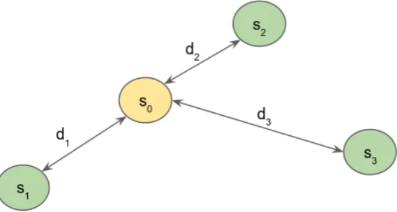
2.1 Three sampled locations (e.g.,s₁,s₂,s₃) are going to be used to estimate the value holds in un-sampled locations₀. The distance between the un-sampled location and each of the sampled locationss₁,s₂,s₃are depicted asd₁,d₂,d₃

respectively. . . 11

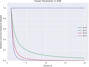
2.2 The relationship between the power parameter pand the inverse distance as a weight in interpolation method, as employed in IDW. Adjusting pto zero means no weights will be implemented and all sample points will be treated equally. As presented in the figure, as pincreases, the influence of the nearest sample points will increase and reduce the influence of the farther ones; resulting a more detail interpolated surface. On the contrary, reducing the power parameter pwill allow more influence of the farther sample points resulting a smoother interpolated surface. . . 12

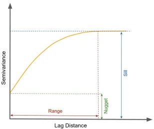
2.3 An example of a variogram with range, nugget, and sill. In variogram, the “range” indicates the shortest distance at which the “sill” is reached. The “range” could be used to identify the size of a search window used in the interpolation methods, where samples with distance larger than the range are spatially independent and not included in the interpolation process. A positive value of the semivariance at lag distance close to zero is called the “nugget”, which also indicates the variance of sampling errors and the spatial

xxiv List of figures

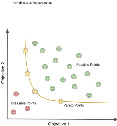
2.4 The plotting of solutions in objective space, where there are two objective functions to be optimised. Infeasible points represent the points in the objective space which violate the constraints (as described in Sub-section 2.2.2). The points in objective space which obey the constraints are called the the feasible points, which also includes the Pareto points. The Pareto Points are the feasible points in objective space which dominate other feasible points but not dominated by the others. The Pareto points also known as the non-dominated points, which collectively will form the Pareto Font (depicted as the yellow line in the figure). . . 20

2.5 The recombination process will exchange the features or characteristics between parents to form a new individual, also known as offspring. The mutation process will randomly alter certain features/characteristics of an individual. Recombination and mutation are utilised in Evolutionary Algo-rithms to maintain variation within the population. . . 22

2.6 A general work-flow in an Evolutionary Algorithm. The initialisation part will generate number of random individuals to form an initial population. The evaluation part takes care two main tasks: evaluate the termination condition and evaluate each individual within the current population in respect to all fitness functions. The selection part in-charge in forming a new population for the next generation. The individuals with higher fitness values will be chosen to form the new population. Variation within the population is

essential in order to explore the search space and to avoid the local optima. In Evolutionary Algorithm, the variation is maintained through mutation and recombination process. . . 23

2.7 A generic ESN architecture which consist of three main components: sensor nodes, base stations, and a server known as Sensor Network Server (SNS). Environmental parameters in the Region of Interest (RoI) are measured and recorded by the sensor nodes. The data is then passed to one or more base stations. . . 26

List of figures xxv

3.2 An example of how an ESN design consisting of five sensor nodes is encoded to form an individual (i.e., a possible solution) and a population (i.e., a set of possible solutions). The Region of Interest (RoI) in this study is gridded as a two dimensional space (151×101) where each cell is indexed. The placement for each sensor node within the RoI is identified by the cell index. In this figure, the fifth sensor node (y5) is placed in index 150 which is

located on the top-right corner of the RoI. . . 41

3.3 Work flow to measure representativeness of an ESN in respect to the Region of Interest (RoI) based on the average spatial temperature. The representa-tiveness is calculated according to the difference between the actual average spatial temperature and the average spatial temperature measured by the deployed sensor nodes over periods of time. . . 47

3.4 Illustration of an overall framework for approach 1. The framework con-sists of two main components: ESN Design Optimisation and Data Quality Assessment. An ESN design with the optimum representativeness (given certain number of sensor nodes) will be searched. For the purpose, a set of historical temperature data is utilised as the dataset in the optimisation process and an Evolutionary Algorithm (EA) is employed to drive the pro-cess. Once the optimum ESN design is found, data quality assessment will be applied toward the design. Such assessment incorporates both gap and noise assessments. . . 51

3.5 An overview of the proposed method in the second approach. The method consist of three main procedures: ESN design optimisation, selecting number of nodes, and selecting node placement. . . 53

3.6 An overview of the ESN design optimisation procedure which incorporates both redundancy and robustness as the objectives to be optimised. . . 54

3.7 Leave One Out Cross Validation (LOOCV) applied in this study. For simplic-ity, the figure presents an example of an ESN formed by three sensor nodes. The LOOCV is conducted by omitting one sensor node in turn while the rest of the nodes are used to predict the omitted node. A spatial interpolation technique (Inverse Distance Weighting) is employed as a method to predict the node. In the end, the prediction errors are calculated as the output of the LOOCV. . . 55

xxvi List of figures

3.9 An overview of the procedure in selecting an ESN design. . . 58

3.10 An illustration of measurement coverage conducted by three mobile plat-forms (e.g., measurement m₁,m₂, and m₃). In every hour, each platform measures the temperature data within the 3×3 gridded area (depicted in a different colour for each platform). Each cell within the gridded area is coded withx₍₁₎,x₍₂₎,· · ·,x₍₉₎, wherex₍₁₎represents the top-left cell andx₍₉₎

represents the bottom-right cell. . . 62

3.11 An example of overlapping in the measurement involving three mobile platforms (e.g., measurement m₁, m₂, and m₃). The overlapped cells are depicted with yellow colour. Measurementm₁andm₂share one overlapped cell (D4); whereas two overlapped cells are shared between measurement

m₂and m₃ (F4 and F5). Such overlapping is possible to occur when there are two or more mobile platforms operated within the RoI at the same time. In this case, the data which is going to be recorded is the averaged data. . . 63

3.12 The movement pattern of a mobile platform applied in this study. The current location of a mobile platform is indicated by pand the array ofqs represents all the possible locations for the next movement. The next location is randomly selected, determined by a unique random seed assigned for each platform. . . 64

3.13 The workflow in the data sampling process up to the construction of two dimensional spatial temperature. As an example, three mobile platforms are employed to explore and collect data within the Region of Interest (RoI). Each platform has a unique random transect which is depicted with a different colour. . . 65

3.14 The figure illustrates how the four average spatial temperature surfaces (one for each season) are transformed into a single sampling cube. This cube is used as a baseline dataset for the optimisation procedure to find the optimum sensor nodes placement which best represent the RoI. . . 66

List of figures xxvii

4.2 A comparison between the number of sensor nodes in each optimum ESN design and its fitness value (i.e., representativeness). The representativeness is measured by the difference (i.e., sum of squared errors) between the actual average spatial temperature and the average spatial temperature produced by the deployed sensor nodes over periods of time. The figure incorporates number of sensor nodes between two and twenty. . . 74

4.3 The impact of certain degree of gaps to the performance of the proposed ESN design (i.e., sensor nodes placement). The gaps are set within the range of 10%, 20%, 30%, and 40% (illustrated by green, red, purple, and yellow lines respectively). For comparison purposes, the performance of the ESN design without gap is also presented using blue line. . . 75

4.4 The improvement promoted by a gap filling process (using Spatial Regression Test) to the ESN design with 40% of gaps. For comparison purposes, the performance of the ESN with no gap, with 40% of gap, and after the gap filling process are illustrated using blue, green, and red lines respectively. . 76

4.5 The impact of certain degree of noise to the performance of the proposed ESN design (i.e., sensor nodes placement). The noise are set within the range of 10%, 20%, 30%, and 40% (illustrated by green, red, purple, and yellow lines respectively). For comparison purposes, the performance of the ESN design without noise is also presented using blue line. . . 77

4.6 Results from noise detection system implemented in this study using temper-ature threshold (as formulated in equation 3.10). Green and red dots are used to mark valid temperature data and noisy data respectively. . . 78

4.7 A demonstration of a single Evolutionary Algorithm (EA) run, showing the evolutionary process of finding a set of near-optimum solutions driven by two fitness functions. The blue marks represent all the solutions (i.e., ESN designs) which have been explored throughout several generations. The red marks represent all the non-dominated solutions (i.e., Pareto Fronts) which have been found so far. . . 79

xxviii List of figures

4.9 A plot of the near-optimum ESN designs optimised for 30 sensor nodes (with respect to both redundancy and robustness as the features to be assessed). Each marker represents a single ESN design. The green markers favour more redundancy (i.e., maximum LOOCV(fˆ)) whereas the the red ones favour more robustness (i.e., minimumRMSE(gˆ)); with the colour gradient in between indicating the balance between the two features. . . 82 4.10 An example of the placement of 30 sensor nodes in the Region of Interest

(RoI). The nodes placement is chosen from one of the markers plotted in Figure 4.9. The background colour represents the elevation in the RoI (in meters). . . 83 4.11 Sampling coverage comparison in two dimensional space and three

dimen-sional cube (i.e., spatial temporal) while exploring the Region of Interest (RoI) using four and nine mobile platforms. Each colour depicted in the figures represents the sampled data from a single mobile platform. . . 84 4.12 Interpolated surfaces of average daily temperature in four different seasons

(e.g., autumn, winter, spring, and summer). The colour-bar on the right hand side indicates the temperature measured in degree Celsius. These surfaces are utilised as a baseline dataset in the optimisation procedure. . . 85 4.13 Optimum placement of sensor nodes given four and nine sensor nodes (as

presented in Figure 4.13a and 4.13b respectively). Each marker represents the placement of one sensor node in the Region of Interest (RoI). . . 86 4.14 ESN representativeness comparison resulting from an experiment conducted

based on three different baseline dataset. The experiment setup was labeled as MS_P04, MS_P09, and MS_P16; indicating the corresponding baseline dataset constructed using four, nine, and sixteen mobile platforms respec-tively. Optimum ESN designs are searched according to a list composed of six different set number of sensor nodes, twenty replication is applied for each set. The representativeness is calculated based on the difference (i.e., root mean squared error) between the actual data and the interpolated data produced by the ESN design. . . 87 4.15 ESN representativeness resulting from four different methods in the design

List of tables

3.1 Parameters setup for Evolutionary Algorithm (EA) implemented in this study. 45 3.2 Parameters used in the experimental setup. MS, HD, RG, and XP are labels

used to represent the experiment setup with the use of mobile sampling, historical data, regular gridding, and expert knowledge respectively. . . 68

Chapter 1

Introduction

Human activity, in the social, economic, health, and safety aspects is impacted by the states of the environment. Favourable environmental conditions contribute in delivering the best outcomes for human activity. Meanwhile, additional regulations are required to deal with harsh environmental conditions to minimise the adversity caused by unfavourable events in the environment (e.g., bush fires, flood, drought). A good understanding of the environmental phenomena (e.g., what happened, when did it occur, what was the magnitude and the duration of the event, how far did its effects spread) will benefit the regulation of human activity. The past and recent records of environmental parameters (e.g., air temperature, relative humidity, wind speed, rain fall, solar radiation) are essential to better understand the environment. In addition, environmental records from a well-monitored region could be used to model the region and forecast its environmental states.

Environmental Sensor Networks (ESN) extend the ability of human to measure and record environmental parameters by greatly increasing the frequency and representation of the measurements, as well as their accuracy [68, 121]. These networks are crucial in support-ing informed decision-maksupport-ing in businesses and communities impacted by environmental changes.

Automated environmental monitoring began with simple automatic logging systems that periodically recorded a number of environmental properties. The lack of communication capability in the early monitoring systems required field scientists to visit the site regularly and collect the recorded data manually [32, 37, 110].

2 Introduction

and communicating their data to a remote data centre without any operator intervention. The networks offer considerably faster and more accurate measurements, compared to the manually accessed logging systems, especially in remote areas which are difficult and sometimes risky or too expensive to reach. These capabilities enable scientists and decision makers to have high quality environmental sensing data which is fundamental for forecast modelling and better decision-making when environmental parameters are relevant.

Predicting changes in the environmental parameters over an extensive region is vital for a number of activities including agriculture and forestry [71, 118, 120], water and air quality assurance [47, 133, 137], logistics [10, 114, 134], tourism and recreation [63, 82], urban development [54, 98, 146], and emergency responses [50, 61]. The application of ESN in these areas will have a significant role to play in improving the quality of human life.

Agriculture and forestry are highly influenced by the changes in the environmental pa-rameters. Agricultural production could be significantly improved by utilising agricultural management strategies with a greater degree of precision (i.e., Precision Agriculture). Pre-cision Agriculture is an emerging area where ESN plays an important role [14, 56]. Apart from the need to increase production, the application of ESN in agriculture and forestry could provide an alternative and realistic means in minimising the use of potentially harmful compounds (e.g., insecticides) in the environment and promoting sustainable agricultural practices. ESN has also been successfully utilised for fire detection systems in forestry [108, 112, 144]. The networks can alert emergency services in the initial detection of the fire before it has spread uncontrollably and destroys hectares of vegetation incurring social, environmental and economic costs. The need to promote better healthcare also motivates the extensive use of ESN to monitor water quality [47, 86, 137] and air quality [51, 109, 133].

In science, ESN not only enables us to find answers to many scientific questions (related to our environment) which could not be answered in the past, but also prompts new questions which have yet to be asked. Furthermore, without ESN, the changes in the earth’s climate would never be readily identified. ESN has been envisioned as a standard component in earth system and environmental sciences which enables scientists to better understand the environment and its phenomena [37, 68].

1.1 Motivation 3

data is utilised to capture the general characteristics of a particular environmental parameter over a certain period of time (e.g., seasonal, annual) [163, 95, 33].

The work presented in this thesis is aimed at contributing to the design aspects of ESN. This work seeks to find the best configuration for sensor nodes with the balance between redundancy and robustness in the networks. Historical records are valuable resource for ESN design, as ESN deployment are most likely to be an evolutionary development. A set of manually monitored, non-integrated sensors may be replaced by an integrated ESN with the designed configuration. In the situation where some of the sensors become non-operative (i.e., sensor failure), there is a necessity to maintain the data quality of the ESN. A graceful degradation in ESN performance is expected. The exploration for the work in this thesis also covers an effort to overcome the unavailability of past measurement records to support the design of ESN. An efficient method is needed to cover a geographical region and gather adequate data in the region that has not been previously monitored.

The following sections in this chapter will present the motivation which signifies the importance of the study, followed by research questions and research objectives that will guide the study presented in this thesis. The overall structure of the thesis will be presented in the last section of this chapter.

1.1

Motivation

Design is a critical process prior to the deployment of Environmental Sensor Networks (ESNs); it is one of the most significant factors in ensuring that the network delivers fit-for-purpose data and is cost-effective. There are two important questions in ESN design:

• How many sensor nodes are needed to serve they serve their purpose as an ESN?

• Where each sensor node should be deployed in the RoI?

The combination between the number of sensor nodes and the size of the RoI will significantly impact the number of possible placement of the nodes in the RoI, where each placement yields different level of representativeness. Complexity is introduced especially when dealing with the requirement to have a fully operational ESN, which meets the application purposes, with the lowest possible number of sensor nodes [19].

4 Introduction

Deploying complex equipment like a sensor node in a remote environment is a very challenging task. There are numerous possible events, starting with harsh environmental conditions to animal activities, which may lead to sensor failure. As sensors start to fail, the usefulness of the network degrades. If an ESN no longer produces the data needed; it is not advisable, or even possible, to rely on data from such a network for decision-making [36, 123, 162]. Having an effective and fully operational ESN is costly and difficult to maintain. Minimising operational costs while delivering useful information is a constant trade-off. In principle, a robust ESN can be achieved by over sampling, at a potentially prohibitive cost. Nevertheless, redundancy in sensor node deployment would also introduce an undesirable increase in costs (e.g., deployment and maintenance costs), which is considered as inefficient in most design practices. For this reason, it is important to find a compromise between ensuring maximum robustness (i.e., fit-for-purpose) and minimising redundancy (i.e., cost-effective). Finding this balance is an optimisation problem.

ESN design is crucial and many studies have been carried out in this space which include several classical parameters such as the number of sensors required to adequately cover a specific area, the position of these sensor nodes, and the required frequency of readings and period of deployment. However, quality assurance and quality control (QA/QC) are neglected in most of ESN design practices. For a balanced design methodology, it is essential to identify an optimum number of sensor nodes (including the placement of each node) which best represents the RoI with low level of redundancy without sacrificing the robustness of the network. Balancing the robustness and the redundancy in the design of an ESN is an interesting yet challenging research problem. The work reported in this thesis is focused on optimising the design of ESN, with particular consideration in the quality of the data supplied by the network. This should result in an ESN that minimises its redundancy (i.e., cost effective) while maintaining the robustness of the network (i.e., greater trust in the data).

1.2

Research Questions

In order to give a clear direction on the study conducted in this thesis, four research questions have been formulated:

• Q1: How to determine the minimum number of sensor nodes to be included in an ESN design?

1.2 Research Questions 5

assist such decision making is essential in order to promote efficiency in ESN design. This research question will guide the study conducted in this thesis in exploring and reviewing the current practices in ESN design in determining the number of sensor nodes. The acquired knowledge can be used as a good foundation to construct and to propose a new method to address the question.

• Q2: How to determine the placement of sensor nodes in an ESN design?

The effectiveness of an ESN design is highly influenced by the the placement of each sensor nodes within an RoI. ESN data is expected to represent the region where the network is deployed. Arbitrary placement of sensor nodes may result to ESN data which fails to represent the RoI. The measured data could be completely unusable and thus the network failed to serve its purpose. A systematic method to find an optimum placement of sensor nodes is needed. This research question paired with Q1 would serve as a guidance for this study to formulate a method in finding an optimum node placement. Such optimum placement would result to an ESN data which best represent the region and eventually promotes the effectiveness of the network.

• Q3: How to improve robustness in an ESN design?

Efficiency is the major focus in current ESN design practices, which mainly deals with minimising the redundancy in the network. However, sensor node failure is common in ESN (i.e., many factors such as harsh environmental conditions could lead to sensor failure). This situation may lead to a condition where an ESN is no longer able to produce data which serves its purpose. Therefore, a certain degree of redundancy might be helpful to preserve the robustness of the network. Finding a balance between redundancy and robustness is needed. This third research question will guide this study to propose a method which incorporates robustness in the design of ESN.

• Q4: How to design an ESN in the absence of historical data?

6 Introduction

1.3

Research Objectives

The work presented in this thesis aims to fill the gap in the current study of ESN design. The proposed method will consider redundancy as a factor to be balanced with robustness to form an optimum ESN design. The following comprises the main research objectives that will be discussed throughout this thesis:

• Formulating the measure of representativeness.

An ESN is deployed in an RoI with the purpose of capturing certain environmental properties in that region. The ESN is expected to produce a set of measured data which best represents the region. Since representation is the main objective of the deployment, it has to be quantifiable. In this case, a clear formulation of representativeness mea-surement is needed. Such a meamea-surement would enable the comparison of a particular ESN design against other ESN designs. This study aims to propose generic method to measure representativeness of an ESN.

• Formulating ESN design as an optimisation problem.

Finding an optimal placement of sensor nodes within an RoI, given a number of nodes, is not a trivial task. Each set of node placements will yield a certain level of representativeness. In this case, the increase in either the number of sensor nodes or the size of an RoI would significantly increase the number of possible node placements in the region (i.e., search space). An optimisation technique which is able to deal with such a large search space is needed. This study aims to construct a method which optimises the sensor node placement, for a given number of nodes, which best represents the RoI.

• Formulating data quality and robustness in ESN design.

Common ESN data quality issues are required to be identified and studied. They have to be clearly defined and well formulated, allowing their impact to the representativeness of an ESN design to be quantified. Some common techniques in overcoming the data quality issues (i.e., data quality controls) are also worthwhile to be explored and studied. These techniques, and the effectiveness of such techniques, should be included when considering ESN design. This study aims to include data quality issues and robustness considerations in the design of ESN.

• Finding a balance between redundancy and robustness in ESN design.

1.4 Thesis Structure 7

to be balanced with robustness. In order to achieve this goal, both redundancy and robustness have to be clearly defined and formulated. Appropriate formulation of redundancy and robustness would enable the trade-off between these two parameters to be quantified. An optimisation technique which could optimise two factors is needed in order to explore all the possible ESN designs. This study aims to propose a method to balance the redundancy and robustness in the design of ESN.

• Formulating an efficient data sampling technique to support the design of ESN.

Historical data related to the past measurement of environmental properties in an RoI is essential not only for the design process prior to the deployment of new ESN, but also for improvement of an existing ESN. Forming an ESN design without any access to historical data has never been a trivial task. It requires a substitution dataset to compensate for the absence of the past measurement data. In this case, a technique to build an initial knowledge regarding the environmental phenomena in the RoI is needed. As an extension, this study aims to propose a method which incorporates mobile data sampling to construct a baseline dataset of an RoI which will be utilised in the ESN design optimisation process.

1.4

Thesis Structure

The rest of this thesis is presented according to the following structure:

Chapter: 2 Literature Review Review of key literature to form a solid foundation for the experimental study being conducted in this thesis. Some key research areas are covered in this chapter including interpolation techniques, optimisation techniques, environmental sensor network, data quality, and design of environmental sensor network.

Chapter 3: Methodology Addresses problem formulation in ESN design within this

8 Introduction

Chapter 4: Results and Validations describes how the proposed method (i.e., as de-scribed in Chapter 3) is applied in the form of experimental study. Results from each experiment are presented and findings are highlighted in this chapter.

Chapter 5: Discussions and Conclusions discusses and concludes several key

Chapter 2

Literature Review

This chapter review some key literature which form a firmed foundation for the experimental study being conducted in this thesis. Some key research areas are covered in this chapter including interpolation techniques, optimisation techniques, Environmental Sensor Network (ESN), data quality, and the design of ESN. The review of the literature is structured as follow:

• Section 2.1 Interpolation Technique

This section describes fundamental concepts in data interpolation, some known inter-polation techniques are also reviewed.

• Section 2.2 Optimisation Technique

Core knowledge in optimisation problem is reviewed in this section, including the general formulation of decision variables and constraints (described in Section 2.2.1 and 2.2.2) which define a search space. This section also covers the formulation of objective function including the concept of domination and Pareto optimal (reviewed in Section 2.2.3, 2.2.4, and 2.2.5) where more than one one objectives are applied.

• Section 2.3 Environmental Sensor Networks (ESN)

This section describes a brief background of ESN including the current development of ESN, the architecture of ESN, and also some applications of ESN (described in Section 2.3.1, 2.3.2, and 2.3.3 respectively).

• Section 2.4 ESN Data Quality

10 Literature Review

• Section 2.5 ESN Design

This section describes how is design matter for having a fit for purpose ESN including the complexity in ESN design. This section also covers some challenges in ESN design, deployment strategy in ESN, and common objectives in the deployment of ESN (describes in Section 2.5.1, 2.5.2, and 2.5.3 respectively).

2.1

Interpolation Techniques

The need of spatially (and also temporally) continuous data of environmental properties are increasing in the environmental sciences. This information is not always readily available, and providing data related to the environmental parameters for any place at any time is a very challenging work for environmental scientists. Ideally, in order to achieve this goal, a considerably dense and interconnected sensor nodes are required to be deployed in the Region of Interest (RoI). This network would enable a fairly accurate estimation of the spatial distribution of the required environmental parameters. However, a network with a high dense sensor nodes is difficult and expensive to deploy and to maintain. Therefore, in most cases, the environmental parameters are measured limited at point locations only, sparse, and not on a regular grid. This often lead to a situation where the data is not available where it is most needed. Developing some methods to estimate the parameters in un-sampled locations is essential to overcome this limitation [1, 15, 101].

Interpolations techniques could be utilised as an alternative to estimate the spatial distri-bution of the climate parameters based on the measurements from the neighbouring sensor nodes. These interpolation techniques are also known as spatial interpolation methods. For-mally, a spatial interpolation technique can be formulised as a mathematical function which capable to predict values at locations in space where there are no measured values available [45]. The uncertainties on the estimated values would increase considerably as the network density decreases. The spatial interpolation techniques are not only been utilised exclusively in environmental science, but also have been utilised widely in many other disciplines. There are several different techniques for spatial data interpolation are available. According to Li and Heap [100] Inverse Distance Weighting (IDW) and Ordinary Kriging (OK) are the most frequently used methods in environmental sciences.

2.1.1

Inverse Distance Weighting (IDW)

2.1 Interpolation Techniques 11

at sampled points weighted by an inverse of the distance from the point of interest (i.e., un-sampled point) to the sampled points (i.e., measured points). This method relies on the assumption that the nearby sampled points point have more similar values than the ones which are further away from the point of interest [52, 132].

The generic formula for IDW can be expressed as follows:

ˆ

Z(s0) =

n

∑

i=1

λiZ(si) (2.1)

Where: ˆ

Z(s₀) is the estimated value located ins₀(i.e., un-sampled point).

Z(s_i) is the measured value located ins_i(i.e., sampled points).

λi is the weight assigned forZ(si)such that∑ni=1λi=1.

n is the number of sampled points used for estimation.

The weights in IDW are calculated according to the following formula:

λi=d_i−p

1

∑ni=1d

−p i

(2.2)

Where:

λi is the weight assigned forZ(si)

d_i is the distance betweens₀ands_i(as illustrated in Figure 2.1)

p is an exponent, also known as the power parameter

n is the number of sampled points included in the interpolation

Fig. 2.1 Three sampled locations (e.g.,s₁,s₂,s₃) are going to be used to estimate the value holds in un-sampled locations0. The distance between the un-sampled location and each of

12 Literature Review

Equation 2.2 suggests that the weights diminish as the distance increases, resulting a higher weight for the nearby sampled points which eventually bring more influence to the estimated value. In this case, the the power parameter pwould greatly affect the accuracy of the prediction. The selection of the power parameter pand sample sizenis arbitrary. Two is the most commonly used value for p, which makes IDW also known as the Inverse Distance Squared (IDS) [115]. Depending on what value been assigned to p, IDW also addressed as “moving average” in the case of pis zero, “linear interpolation” when pis 1 and “weighted moving average” when pis not equal to 1 [99]. The relationship between weight, distance, and power parameter in IDW is presented in Figure 2.2

Fig. 2.2 The relationship between the power parameter pand the inverse distance as a weight in interpolation method, as employed in IDW. Adjusting pto zero means no weights will be implemented and all sample points will be treated equally. As presented in the figure, as p

2.1 Interpolation Techniques 13

2.1.2

Ordinary Kriging (OK)

Ordinary Kriging (OK) is one of the geostatistical methods to estimate the value in an un-sampled location based on the measured values from nearby un-sampled locations [38]. Similar to IDW, OK also implements weights in its calculation. The generic formula of OK is also similar to IDW as described in Equation 2.1. In contrast to IDW, OK assigns weights to its sample points not only based on their distances, but also based on the spatial variability structure. In OK, spatial and statistical relationships are considered as the basis to constructs weights [151].

Semivariance is employed to measure the the degree of spatial dependence between sample locations. In terms of calculation, semivariance is simply a half of the variance of all available sample points in space with a constant distance apart. In geostatistics, the semivariance is formalised as follows:

γ(h) = 1

2N(h)

N(h)

∑

i=1

(Z(s_i)−Z(s_i+h))2 (2.3) Where:

γ(h) is the semivariance with lag distanceh.

h is the lag distance between two sample points.

N(h) is the number of sample points which have lag distance ofhwith the other sample points.

Z(s_i) is the value measured in sample points_i.

The semivariance can be estimated from the data by employing certain fitted function (i.e., variogram modelling) and the plotting of the fitted data (i.e., variogram). This modelling and estimation is essential for structural analysis and spatial interpolation [24]. Figure 2.3 shows an example of variogram plotting.

The weights in OK are obtained by minimising the variance in OK prediction error

[Zˆ(s0)−Z(s0)], also known as “Kriging variance”, which is formalised as follows:

σ_e2=

n

∑

i=1

λiγ(xi,x0) +θ (2.4)

14 Literature Review

Fig. 2.3 An example of a variogram with range, nugget, and sill. In variogram, the “range” indicates the shortest distance at which the “sill” is reached. The “range” could be used to identify the size of a search window used in the interpolation methods, where samples with distance larger than the range are spatially independent and not included in the interpolation process. A positive value of the semivariance at lag distance close to zero is called the “nugget”, which also indicates the variance of sampling errors and the spatial variance at

shorter distance than the minimum sample spacing [99].

σ_e2 is the Kriging variance.

n is the number of sample points.

λi is the proposed weight for sample pointsisuch that∑n_i=1λi=1.

γ(xi,x0) is the semivariance between the values at sample location si and

un-sampled location s₀. Such value can be obtained from the fitted vari-ogram.

θ is the Lagrange multiplier required for minimisation.

2.2

Optimisation Techniques

2.2 Optimisation Techniques 15

required to be satisfied, the task of finding the optimal solution is called single-objective optimisation. It follows then that if there is more than one objective function that needs to be satisfied, the task of finding one or more optimum solutions is called multi-objective optimisation [22, 42]. Further, Coello et al. [35] provides a clear definition of multi-objective optimisation problem as:

“The problem of finding a vector of decision variable values which satisfies con-straints and optimises a vector function whose elements represent the objective functions. These functions form a mathematical description of performance criteria, which are usually in conflict with each other. Hence, the term ‘optimise’ means finding such a solution which would give the values of all the objective functions acceptable to the decision maker.”

Most problems in real world applications have multiple objectives, which are possibly conflicting with each other. By optimising one objective, one may be sacrificing the other objectives. A simple example can be found in computing equipment purchase decisions. People in general want to have computing equipment with high performance. However, people also want to save their money and spend less. In this case, the objective of having the computing equipment with the best performance cannot be achieved without abandoning the objective of spending less money in purchasing. On the other hand, the objective of spending less cannot be achieved without sacrificing the objective of having computer equipment with the best performance. The objectives in the purchasing decision are in conflict with each other.

2.2.1

Decision Variables

The decision variables in optimisation problems are the numerical values, which are chosen in such a problem. In mathematical notation, the variables can be represented as:

x_i,i∈ {1,· · ·,n} (2.5) Or it can also be noted as a vectorxofndecision variables as follow:

¯

x= [xi,· · ·,xn] (2.6)

16 Literature Review

2.2.2

Constraints and Decision Variable Bounds

Constraints in optimisation problems are the restrictions or limitations introduced by the environment or resources, such as physical limitations, time restrictions, processing power limitations, and several other kind of limitations. Certain solutions can be considered acceptable when these solutions can satisfy all the available constraints. In mathematical notation, these constraints can be represented either in mathematical inequality:

g_i(x¯)≤0,i∈ {1,· · ·k} (2.7) or equality as follows:

h_j(x¯) =0,j∈ {1,· · ·l} (2.8) In this case,krepresents the number of inequality constraints andlrepresents the number of equality constraints.

Letnbe the number of decision variables, then the number of inequality constraintsk

cannot be greater than or equal ton. In other word,kmust be less thann(k<n). Since the degree of freedom in multi-objective optimisation problem is defined as n−p, therefore, the optimisation problem withk≥nis considered as over constrained and there is no more flexibility or any degree of freedom for optimising.

In addition to the constraints, there are also decision variable bounds. In mathematical notation, the variable bounds can be expressed as follows:

x_i(L)≤xi≤x_i(U),i∈ {1,· · ·,n} (2.9)

Where:

x(_iL) is the lower bound value for decision variablei.

x(_iU) is the upper bound value for decision variablei.

n is number of decision variables to form a solution.

These variable bounds restrict each decision variable to take a value only in the range between the lower value and the upper value. The bounds also represent a decision variable spaceDknown as decision space.

2.2 Optimisation Techniques 17

2.2.3

Objective Function

In the study of optimisation problems, an objective function is defined as the computable function of a vector of decision variables, which is used as a criterion to evaluate a certain solution in order to know how good the solution is. In real world optimisation problems, some functions are required to be minimised while other functions are required to be maximised. Moreover, in multi-objective optimisation problems, these functions in many cases are in conflict with each other. Optimising a particular objective function may sacrifice the other objective functions. These objective functions may be measured using the same measurement units (i.e., commensurable) or the functions may also be measured using different measurement units (i.e., non-commensurable). In mathematical notation, the objective functions can be represented as follows:

f_i(x¯),i∈ {1,· · ·,m} (2.10) Where:

f(x¯) is the objective function to be optimised given ¯xas the parameter. ¯

x is a vector of decision variables, also known as a solution.

m is the number of objective functions being solved in the multi-objective optimisation problem.

Since there would be more than one objective function available in a multi-objective optimisation problem, these functions will form a vector function, which can be expressed in mathematical notation as follows:

f(x¯) = [f1(x¯),· · ·,fm(x¯)] (2.11)

Referring to the notation, the goal in a multi-objective optimisation problem can clearly be seen as the problem of optimising themnumber of objective functions simultaneously. The optimisation process itself can be maximising the values of allmobjective functions, or minimising the values of allmobjective functions, or even in some cases could be combining the maximisation and the minimisation values of thesemobjective functions. Since the task in multi-objective optimisation problems is about optimising a vector of objectives instead of a single-objective, multi-objective optimisation is also known as vector optimisation.

18 Literature Review

objective function by negative one (−1). The same thing works vice versa, depends on the implementation of the algorithm.

2.2.4

Concept of Domination

The concept of domination is widely applied in the field of multi-objective optimisation problems in order to compare two solutions. Two solutions are compared to see whether one solution dominates the other or not.

Let ¯xand ¯ybe two solutions in a multi-objective optimisation problem. Solution ¯xis said to dominate solution ¯y, or in mathematical notation expressed as ¯x_≼y¯, if and if only it complies with these two domination conditions:

1. Solution ¯xis no worse than solution ¯yin all objective functions;

2. Solution ¯xis strictly better than solution ¯yin at least one objective function.

In the case of minimisation as an optimisation problem, these domination conditions can be expressed in mathematical notation as follows:

¯

x= [x₁,· · ·,x_n]

¯

y= [y1,· · ·,yn]

¯

x_≼y¯⇔(∀i: f_i(x¯)≤ f_i(y¯))∧(∃i: f_i(x¯)< f_i(y¯),i∈ {1,· · ·,m})

(2.12)

Where nrepresents the number of decision variables that construct a solution and m

represents the number of objective functions being solved in a multi-objective optimisation problem.

Apart from representing solution ¯xdominating solution ¯y, this mathematical notation also implies that:

1. Solution ¯yis dominated by solution ¯x, 2. Solution ¯xis non dominated by solution ¯y, 3. Solution ¯xis non inferior to solution ¯y.

2.2.5

Pareto Optimal

2.2 Optimisation Techniques 19

than just a single objective function require to be satisfied and in most cases, the objective functions are in conflict with each other. Finding a single global optimal solution in the decision variable spaceDis nearly impossible. In multi-objective optimisation problems, instead of looking for a single solution, the focus is looking for a trade-off among the objective functions. For this purpose, optimality of a solution needs to be redefined properly in order to respect the integrity of each objective function [34, 43, 64].

The concept of domination is utilised in the multi-objective optimisation problem and it is also known as the Pareto dominance. All possible pairwise comparisons can be performed for a given finite set of solutions in order to find which solutions are non-dominated with respect to each other. The set of non-dominated solutions that is left has the property of dominating all other solutions apart from the solutions which belong to this set. Any member in the entire search space of solutions does not dominate these solutions. In other words, the set of non-dominated solutions are better compared to all other solutions [79, 147].

In multi-objective optimisation problem, the set of non-dominated solutions is also known as Pareto Optimal Set. In mathematical notation, the Pareto Optimal Set can be expressed as follow:

P∗={x¯∈D|¬∃x¯∗∈D: f(x¯∗)_≼ f(x¯)} (2.13) Where:

P∗ is the set of non-dominated solutions, also known as Pareto optimal set. ¯

x is a solution (i.e., a vector of decision variables). ¯

x∗ is an optimal solution.

D is the search space where a solution could be found/formed.

f(x¯) is the objective function to be optimised given ¯xas the parameter.

The global Pareto Optimal Set can be defined as the non-dominated set of the entire feasible search spaceS. Often the globally Pareto Optimal Set is simply referred to as Pareto Optimal Set.

Furthermore, by plotting the Pareto Optimal Set in objective space, the non-dominated vectors are collectively known as the Pareto Front. Figure 2.4 shows an example of Pareto Front with two objective functions. In mathematical notation, Pareto Front can be represented as follow:

20 Literature Review

PF∗ is the Pareto Front.

P∗ is the set of non-dominated solutions, also known as Pareto optimal set. ¯

x is a solution (i.e., a vector of decision variables).

u is a value produced by the objective function f given a vector of decision variables ¯xas the parameter.

2.2 Optimisation Techniques 21

2.2.6

Evolutionary Algorithms

In order to solve multi-objective optimisation problems, the Operations Research community has developed several approaches since the 1950s based on a variety of mathematical pro-gramming techniques. However, there are several limitations in mathematical propro-gramming techniques when dealing with multi-objective optimisation problems. Most of them only produce a single solution for each run; therefore in order to produce a Pareto Optimal Set, several runs are required. Moreover, mathematical programming techniques in general are susceptible to the shape and continuity of the Pareto Front [35, 57].

Evolutionary Algorithms are computer programs that mimic natural evolutionary prin-ciples, which are inspired by Charles Darwin, in order to solve complex searching and optimisation problems. In Evolutionary Algorithms there would be a number of artificial creatures, known as individuals, which are generated to search over a particular problem space. Individuals continually compete against each other in order to discover the optimal areas from the predefined search space. Gradually, over some periods of time, the most successful individuals evolve to discover the optimal solution [28, 43, 64].

In contrast to the mathematical programming techniques, which in general only produce a single solution for each run, Evolutionary Algorithms can find several members of the Pareto Optimal Set in a single run. Evolutionary Algorithms are also less susceptible to the shape or continuity of the Pareto Front.

The individuals in Evolutionary Algorithms are commonly represented by strings or vectors that have a fixed length. Every individual encodes a unique possible solution to address a particular problem. In Evolutionary Algorithms, a set of individuals is known as a population.

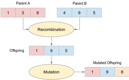
The Evolutionary Algorithm is started with an initial population consisting of a particular number of randomly generated individuals. A fitness value is then calculated for each individual. In order to generate the fitness value, each individual is decoded to produce a possible solution to the problem. The fitness function will calculate the solution value to produce a fitness value for the corresponding individual. The individuals with higher fitness values represent better solutions to address the problem, compared to the ones with lower fitness values. This initial process is followed by the main iterative cycle, which consists of two main operations, mutation and recombination [35]. Figure 2.5 presents the recombination and mutation process which is commonly used in Evolutionary Algorithms to maintain variation within the population.

22 Literature Review

Fig. 2.5 The recombination process will exchange the features or characteristics between parents to form a new individual, also known as offspring. The mutation process will randomly alter certain features/characteristics of an individual. Recombination and mutation are utilised in Evolutionary Algorithms to maintain variation within the population.

members of the new population. This new population will be treated as the current population in the next iteration cycle. In order to control the growth of the population, a similar approach to the natural evolutionary strategy (the survival of the fittest) is applied and the individuals start competing against each other. This kind of approach in Evolutionary Algorithms is known as the selection process. The fitness value is used as the basis for the selection process. The individuals with better fitness values have more chance of being selected as parents (to produce offspring) and also to be selected to form a new population. Such iterative process will run until certain termination condition is satisfied. Maximum number of generation is a commonly used termination condition in Evolutionary Algorithms. Figure 2.6 shows the overall process in Evolutionary Algorithms.

According to Deb [42], in order to solve multi-objective optimisation problems, there are four main primary goals that can be identified in Evolutionary Algorithms:

2.3 Environmental Sensor Network (ESN) 23

Fig. 2.6 A general work-flow in an Evolutionary Algorithm. The initialisation part will generate number of random individuals to form an initial population. The evaluation part takes care two main tasks: evaluate the termination condition and evaluate each individual within the current population in respect to all fitness functions. The selection part in-charge in forming a new population for the next generation. The individuals with higher fitness values will be chosen to form the new population. Variation within the population is essential in order to explore the search space and to avoid the local optima. In Evolutionary Algorithm, the variation is maintained through mutation and recombination process.

2. Continually make algorithmic progress towards the Pareto Front in the objective function space.

3. Maintain diversity in the Pareto Front Set and the Pareto Optimal Set.

4. Provide a large enough Pareto Optimal Set for the decision maker.

2.3

Environmental Sensor Network (ESN)

24 Literature Review

node actively communicates its own observed data to nearby sensor nodes. Moreover, these interconnected sensor nodes also have a capability to process and communicate their data to a remote data centre without any operator intervention. These monitoring systems are known as Environmental Sensor Networks (ESNs), which enable long-term environment monitoring at scales and resolutions that are difficult to achieve with conventional observation methods [32, 37, 68, 110, 121].

2.3.1

Development of Sensor Networks

The deployment of cheap and smart devices in large numbers with multiple on-board sensors, which connect together through wireless networks and the Internet, offers tremendous and unprecedented opportunities for collecting information on a wide range of entities of interest. Even though the research on sensor networks was initiated for military purposes, further development in low-cost sensors and communication networks has broadened the potential application of sensor networks from infrastructure security to industrial sensing. The sensor networks could be deployed in houses, offices, hospitals, cities, and the environment to get a better understanding and to control surrounding conditions [32].

Three different areas of study are involved in the development of sensor networks technology: sensing, communication, and computing, which includes hardware, software, and algorithms. Development in sensor networks has been driven by both the combined and separate advancement in each of these three research areas. The collaboration can clearly be seen from the three main components of a sensor node: sensors as sensing devices, data processing unit, and communication unit which enable it to establish untethered communication at short distance [4, 32, 92].

An on-board processing unit enables each sensor node in sensor networks to conduct in-situ data processing. Therefore, rather than sending the raw data to the base station, each node can handle simple data processing locally and transmit only the required data to the base station. This cooperative effort of sensor nodes is one of the unique properties of sensor networks [3, 121]. Furthermore, the advancement in Micro-Electro-Mechanical Systems (MEMS) brings a substantial contribution in the miniaturisation of sensor nodes. MEMS has

revealed the possibility of producing significantly smaller sensor nodes with multifunctional capability and low power consumption. The fast growth in the development of MEMS offers a wide range of promising future applications, considering the relatively low manufacturing cost offered by this technology [69].

2.3 Environmental Sensor Network (ESN) 25

and memory capacity. In a sensor network, sensor nodes are densely deployed in large num-bers and the network topology changes frequently. The individual nodes are also prone to failure. Considering the large number of sensors and the communication overhead, having a global identification for sensor nodes, which is commonly found in traditional networks, may not be possible. Broadcast communication is also employed by most sensor nodes, whereas ad-hoc networks mainly rely on point-to-point communication. These conditions make the technologies that are currently available for ad hoc networks not well suited to the unique requirements of sensor networks. Recently, there have been many researchers working in this area in order to fulfil these requirements [4].

Energy has been recognised as one of the main challenges in ESN, especially for those deployed in remote locations. The recent development in energy harvesting technology could be considered an important element supporting the advancement in ESN. This particular technology enables electronic devices to produce some amount of energy (electrical power) from its ambient environment such as by utilising propagated radio waves, wind flow, sunlight, or mechanical vibration [12].

2.3.2

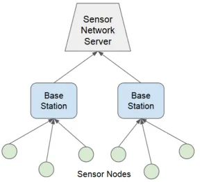
Sensor Network Architecture

A generic ESN architecture is constructed with three main component: sensor nodes, base stations, and a sensor network server (as presented in Figure 2.7). Sensor nodes gather the environmental raw data and simple data processing might be present in each node. The pre-processed data will be passed to one or more base stations for further data processing. Sensor Network Server (SNS) acts as a data repository where data from several base stations is aggregated. More sophisticated data processing will also be handled at this stage. In order to provide seamless access to the environmental information for external users, a web service is utilised as an interface between the SNS and the users. Moving up the hierarchy from the sensor nodes to the SNS, there is an increase in computational capability, data storage capacity, and power availability. In general, the sensors nodes and the base stations in ESN may be able to serve for a few months only. This is due to the power supply limitation and harsh environmental conditions [4, 3, 5, 136].

2.3.3

Applications of ESN