Natural length scales of ecological systems: Applications at community and ecosystem levels

Insight, part of a Special Feature on Catastrophic Thresholds, Perspectives, Definitions, and Applications

Natural Length Scales of Ecological Systems: Applications at Community

and Ecosystem Levels

Craig R. Johnson

ABSTRACT. The characteristic, or natural, length scales of a spatially dynamic ecological landscape are the spatial scales at which the deterministic trends in the dynamic are most sharply in focus. Given recent development of techniques to determine the characteristic length scales (CLSs) of real ecological systems, I explore the potential for using CLSs to address three important and vexing issues in applied ecology, viz. (i) determining the optimum scales to monitor ecological systems, (ii) interpreting change in ecological communities, and (iii) ascertaining connectivity between species in complex ecologies. In summarizing the concept of characteristic length scales as system-level scaling thresholds, I emphasize that the primary CLS is, by definition, the optimum scale at which to monitor a system if the objective is to observe its deterministic dynamics at a system level. Using several different spatially explicit individual-based models, I then explore predictions of the underlying theory of CLSs in the context of interpreting change and ascertaining connectivity among species in ecological systems. Analysis of these models support predictions that systems with strongly fluctuating community structure, but an otherwise stable long-term dynamic defined by a stationary attractor, indicate an invariant length scale irrespective of community structure at the time of analysis, and irrespective of the species analyzed. In contrast, if changes in the underlying dynamic are forcibly induced, the shift in dynamics is reflected by a change in the primary length scale. Thus, consideration of the magnitude of the CLS through time enables distinguishing between circumstances where there are temporal changes in community structure but not in the long-term dynamic, from that where changes in community structure reflect some kind of fundamental shift in dynamics. In this context, CLSs emerge as a diagnostic tool to identify phase shifts to alternative stable states associated with loss of resilience in ecological systems and thus provide a means to interpret change in community composition. By extension, comparison of the CLSs of ostensibly similar communities at different points in space can reveal whether they experience similar underlying dynamics. Analysis of these models also reveals that species in the same community whose dynamics are largely independent indicate different length scales. These examples demonstrate the potential to apply CLSs in a decision-support role in determining scales for monitoring, interpreting whether change in community structure reflects a shift in underlying dynamics and therefore may warrant management intervention, and determining connectivities among species in complex ecological systems.

Key Words: attractor reconstruction; characteristic length scale; community change; connectivity;

monitoring; natural length scale; scaling threshold

INTRODUCTION

Important Issues in Applied Ecology

Three important challenges in applied ecology are (1) determining the appropriate spatial scales for monitoring communities and ecosystems, (2) interpreting temporal change in community and

to yield different patterns and behaviors (Wiens 1989, Levin 1992). Even if the scales at which particular processes manifest are known, it is frequently the goal of ecosystem monitoring to detect trends in behavior at a system level. If identifying system trends is desirable, then it is important to sample at the scale that most clearly reflects the underlying deterministic dynamics (Rand and Wilson 1995, Keeling et al. 1997, Pascual and Levin 1999, Wilson and Keeling 2000). If the sampling scale is too small the deterministic or “trend” signal will be swamped by noise, whereas if it is too large then trends in different areas of a landscape that are essentially independent are averaged and trivial. However, ecologists typically make decisions about scales for monitoring based on a mix of expedience (what is practicable) and experience (what seems to work). More objective means to identify appropriate scales for monitoring have been elusive.

A related challenge is the interpretation of temporal change in community or ecosystem structure. It is vital that ecologists (and managers) are able to distinguish between shifts in community composition attributable to the inherent or “natural” fluctuations of a system with otherwise stable long-term dynamics, and those reflecting some kind of fundamental change in the underlying dynamics (Rand and Wilson 1995). Developing this capacity will help minimize the conflicts and confusion that arise from disagreement about the existence and meaning of particular ecological change (e.g., see Fabricius and De’ath 2004), especially in the context of environmental impact, which has far-reaching implications for managers and other stakeholders in the natural environment.

Survey protocols developed for analysis by particular statistical models, such as the “beyond BACI” designs (Underwood 1994), can be helpful to determine whether community structure and temporal variation at a particular site of interest might differ from that of putative control sites (but see Stewart-Oaten and Bence 2001). However, ignoring deeper philosophical issues with this kind of hypothesis-testing approach (e.g., Berger et al. 1997, Johnson 1999, Eberhardt 2003, Hobbs and Hilborn 2006), even these relatively elaborate designs shed only limited light on a more fundamental interpretation of change. Even when the dynamics at several sites are described by the same attractor, community structure and patterns of community change at one site may differ

substantially from that at others simply because the dynamics in different areas of space are out of phase. In other words, the pattern of temporal change in community structure might be asynchronous but otherwise similar at all sites. Although ecologists have long recognized that communities at different sites might be at different stages of a particular dynamic (e.g., Watt 1947), the challenge to interpret an observed temporal change is perennial. Particularly where changes in community structure are potentially linked to management responses, it is not sufficient to know that change has occurred, but it is important to identify whether the change is the result of a fundamental shift in underlying dynamics (Rand and Wilson 1995) and, ultimately, its underlying cause (e.g., Underwood 1996, Fabricius and De’ath 2004).

The concept of connectivity (i.e., interaction strength) among species is a central theme in both theoretical and empirical community ecology (e.g., see Laska and Wootton 1998) to the extent that it is covered in many ecological texts (e.g., Ricklefs 1990, Pimm 1992, May 2001). In applied work, knowledge of connectivity is important because it provides insight into the “downstream” or “ripple” effects of changes in abundance of particular species. Patterns of connectivity are, of course, fundamental to work concerned with trophic cascades and issues of “top-down” vs. “bottom-up” control of community dynamics (e.g., Schmitz et al. 2000, Bascompte et al. 2005, Borer et al. 2005). However, most empirical work to date has usually managed to identify connectivities as a result of direct interactions between pairs of species, and in short interaction “chains” or simple food webs (e. g., Frank et al. 2005). In more complex systems, the connectivity between species resulting from indirect interactions can be difficult to detect because effects of fluctuations in one species on others in the system can be complex (Bruno and O’Connor 2005). Proxies of direct and indirect interactions such as stable isotopes (e.g., Connolly et al. 2005) and fatty acids (e.g., Phillips et al. 2003) have been helpful to identify more diffuse connectivities, but only for trophic interactions among species. For non-trophic interactions, such as competition, identifying connectivities in the dynamics of species that interact indirectly can be difficult.

identifying connectivity among species is possible through consideration of the characteristic length scales (CLSs) of ecological systems. In this paper, I briefly review the concept of CLSs and, by way of example, analyze the dynamics of spatially explicit stochastic individual-based-models to show that CLSs may be useful to address these issues in applied ecology.

A Brief Introduction to the Concept of CLSs

Scaling thresholds in the description of spatial pattern and heterogeneity in species’ abundances in ecological systems have been recognized for over five decades (e.g., Greig-Smith 1952, Kershaw 1957). This early work showed the importance of using an optimum sampling scale, identified using a type of variance spectrum, to identify and describe spatial pattern. It was the genesis of a suite of techniques, all based on variance spectra of various kinds, to identify “natural scales” of ecological systems (Tyre et al. 1997 present a useful summary of much of this work). However, all of these approaches were based on assumptions that the mean abundances of species were invariant in time and, usually, in space, and so although these methods could provide insight into ecological models with these properties (e.g., De Roos et al. 1991, Tyre et al. 1997), their application to real ecological systems was limited. Indeed, in attempting to apply several techniques to data from real systems, Tyre et al. (1997) concluded that the search for CLSs in real systems “seems to be futile.”

Two other research groups tackled the problem from a different perspective, acknowledging at the outset that real systems were anything but steady state, and much more likely to be characterized by complex oscillatory non-linear dynamics. Keeling et al. (1997) and Pascual and Levin (1999) applied techniques from non-linear time series, using space–time data describing the dynamics of a single species to reconstruct the attractor of its system in a phase space of minimum dimensions topologically equivalent to the attractor of the full system (Takens 1981). The approach developed from the earlier work of De Roos et al. (1991) and Rand and Wilson (1995), who examined how variance changed with the size of “windows of observation” in two-dimensional spatial systems with stationary means. This approach assumes that the system has an underlying deterministic dynamic and that the species in the system are dynamically linked, either

directly or indirectly. Providing these assumptions are met, the technique enables building the attractor in phase space from time delay coordinates of a single species, i.e., the dynamics of the whole system are predicted from observations through time of a single variable in the system.

The attractor reconstruction is then used to make predictions of the time series, and the predicted and actual trajectories are compared to quantify the magnitude of the error in the prediction. The approaches of Keeling et al. (1997) and Pascual and Levin (1999) differ largely in how they define this “prediction error.” Keeling et al. (1997) define a quantity termed “error-X” whereas Pascual and Levin (1999) use a metric they call “prediction-r2,” and they are both measures of variance of some form. Error-X is a scaled error variance, whereas prediction-r2 is analogous to R2 in standard linear regression.

Recent Developments and Application to Real Ecological Systems

The single largest problem with the techniques of Keeling et al. (1997) and Pascual and Levin (1999) is that they require long time series of highly spatially resolved data to reconstruct the system attractor. Time series of at least ~1000 “maps” of a landscape, but preferably several thousands of maps, are required. For this reason, these approaches can only be applied to models of ecological systems because this kind of data is not available for natural systems. Habeeb et al. (2005) addressed this problem and showed that by substituting space for time, the attractor reconstruction can be undertaken from very short time series of as few as three consecutive maps, or even by using a single map. They examined several spatially explicit models and showed that estimates of the CLS obtained from their technique based on short time series were identical to those based on the original work using long time series.

Subsequently, it has been shown that the short time series approach yields consistent and unambiguous estimates of the CLS for real ecological systems. Moreover, as predicted by the underlying theory, the estimate of the CLS is similar irrespective of the species used for the attractor reconstruction, even though different species in the ecological community they examined have vastly different taxonomic affiliations, life history characteristics, abundances, and population dynamics (Habeeb 2005; R. Habeeb, C. Johnson, S. Wotherspoon, unpub. ms.). This result emphasizes that the CLS is truly a system-level measure.

It is worth noting that in systems with more complex dynamics, the prediction-r2 spectrum reveals secondary length scales of greater magnitude than the “primary length scale” indicated by the point where the spectrum first begins to flatten. These secondary scales are thought to reflect the scale of emergent dynamics that arise through some form of self-organization in the system (Habeeb et al. 2005).

These developments are exciting because they show that real ecological communities demonstrate unambiguous CLSs, and that they can be estimated reliably. Importantly, because (by definition) the CLS indicated by the prediction-r2 spectrum defines the optimal scale at which to observe a system to identify the underlying deterministic trend, the technique provides an objective means to assist

decisions about optimal scales for monitoring real ecological systems. The technique can also be applied at the habitat level, examining changes in the spatial arrangement of interacting habitats, to identify the scale at which trends in habitat dynamics are most readily identified (Habeeb et al. 2007). This information, whether at the level of species or habitat types, is useful to both managers and applied ecologists. However, it needs to be reiterated that the CLS is not necessarily the scale at which to observe a particular ecological process of interest, because different processes with large effects on ecological dynamics operate across a large range of scales. Rather, the CLS is a system level property that defines the scale at which to observe the system given the myriad processes that influence its dynamic.

Applying CLSs to Interpret Change and Assess Connectivity in Ecological Systems

Given developments of the technique that enable application to real ecological systems (Habeeb 2005, Habeeb et al. 2005, 2007; R. Habeeb, C. Johnson, S. Wotherspoon, unpub. ms.), it becomes useful to examine whether consideration of CLSs can assist with identifying connectivities in ecological systems and with the vexed issue of interpreting ecological change. Based on the underlying theory (Keeling et al. 1997, Pascual and Levin 1999, Habeeb et al. 2005) it can be predicted that:

1. Whereas the community structure of an ecological system might show large fluctuations, if the underlying dynamic of the community is invariant then analysis of the system should yield identical values of the CLS irrespective of community structure at the time of analysis or the nature of the species examined;

2. Changes in the CLS of a community reflect a fundamental shift in the underlying dynamics; and

3. If two species in the same community indicate dissimilar length scales, then their dynamics are largely independent.

and show that, with some caveats, these predictions hold. These examples demonstrate the potential to apply this approach to real ecosystems, and thus define a need to obtain robust spatial ecological data.

METHODS

General Formalism of Spatially Explicit Models

The models examined in this study are all produced using the Compete© software (available at http://w ww.zoo.utas.edu.au/CJPblist/cj_sftwre.htm, inclu-ding user manual and outline of architecture). The basic structure is a stochastic individual-based system that simulates spatial competition between sessile colonial organisms. The “landscape” is a coupled lattice on which species can recruit, grow, produce propagules, and die. Each cell on the landscape is either empty or occupied by a single species. The community develops depending on the rates of recruitment, growth, and mortality of each species (defined by the probabilities of each event), and the nature of the outcome of pairwise interactions, which are specified by the probability of a win, loss, or standoff in any given encounter. Recruitment can only occur to bare space, whereas mortality is described by both the likelihood of a mortality event and the size of the mortality (i.e., number of contiguous cells that die). Random disturbances are possible, defined by the frequency, shape, and size of events that clear occupied cells. Updating of the landscape is synchronous.

Growth and interaction outcomes are developed as cellular automata. For an unoccupied cell, a random neighbor in its von Neumann neighborhood (i.e., cells to its north, south, east, and west) is chosen, and if the selected neighboring cell is occupied by species Si, then Si grows into the empty cell with a probability specified by its growth rate (gi). By this mechanism, “bays” fill in more quickly than “headlands” advance, and so colonies in bare space develop an approximately circular morphology. Updating the state of an occupied cell is slightly more involved. The cell of interest Ci chooses a random neighbor Cj (also in its von Neumann neighborhood), and Cj overgrows Ci with the probability Pr[Cj > Ci] · gj, where Pr[Cj > Ci] defines the probability of Sj winning in an encounter with

Si, and gj is the growth rate of Sj.

These kinds of spatially explicit models can closely represent the dynamics of real ecological systems

(Wootton 2001, Dunstan and Johnson 2005), and often demonstrate complex behaviors including non-linear dynamics and spatial self-organization (e.g., Johnson 1997, Johnson and Seinen 2002, Habeeb et al. 2005). An important consequence of spatialization of models in this way is the emergence of stability not evident in their mean-field counterparts (e.g., Hassel et al. 1991, Nowak and May 1992, Johnson 1997).

In all models in this paper, landscapes are toroidal (zero boundary conditions) to minimize edge effects, and are 300 x 300 cells in dimension. Initial recruitment to a bare landscape covers a total of 10% of the landscape and there is an equal number of recruits of each species. For simplicity (unless stated otherwise), there is no disturbance, no ongoing recruitment, no endogenous mortality of colonies on the landscape, and each species i grows at the maximum possible rate gj = 1.0. The qualitative results of the analyses are not dependent on these simplifications. In those models where ongoing recruitment is allowed (see below), recruitment is from an open system, i.e., propagules of all species are equally available independent of the cover of species on the landscape.

Specific Structure of Models to Address Predictions

The predictions are examined by studying the length scales and behaviors of several model systems, and the specific structure of the models is outlined under each prediction below. In describing the network topologies, Si > Sj indicates that species i overgrows and displaces species j, and that this outcome occurs in 100% of encounters between Si > Sj unless stated otherwise.

Prediction 1. The CLS of a community showing changes in structure through time will not change if the underlying dynamic is constant.

Fig. 1. Dynamics of a three-species system (A) demonstrating a stationary attractor but characterized by strong oscillations of the two dominant species (Sred and Sblue). Even though the landscape at different times might be dominated by either Sred (B = landscape at 5880 generations) or Sblue (C = landscape at 19 350 generations), prediction-r2 spectra derived from analysis of landscapes at these two times,

Three-species model: The network topology of the

model is S3 > S2 > S1, which can be viewed as representing a trophic hierarchy with S1 as a primary producer, S2 as a herbivore, and S1 as a carnivore (there is a standoff between S1 and S3 wherever they meet on the landscape). S3 has a likelihood of mortality of 0.0005 per cell, and if a mortality event is initiated the extent of mortality is only a single cell. Cells cleared through mortality can attract recruits. Each species has an equal chance of being selected as a potential recruit and, once selected, recruitment rates are determined by the probabilities

S1 = 1.0, S2 = 0.005, and S3 = 0.

Prediction 2. A shift in underlying dynamics will be reflected as a change in the CLS.

Here, four models are considered to examine several different ways in which the dynamics of a community might change. The first two are based on the same five-species system in which a shift in the “physical environment” changes the characteristics of some species in relatively minor ways that, however, have a large effect on the community dynamics. In one case, the growth of one species is reduced by 25% (Figs. 2A, 3), and in the other, the nature of the interaction between two of the species (S1 and S2) changes so that instead of S1 overgrowing

S2 in 100% of encounters, S1 displaces S2 in 60% of cases, otherwise S2 overgrows S1 (Figs. 2B, 4).

The third is a 20-species model in which all species co-exist indefinitely because propagules of all species arrive at a constant rate to colonize small patches cleared by disturbance, i.e., the landscape exists in an “open recruitment” system. The dynamics are changed when the “open” recruitment, i.e., constant supply of propagules, ceases (Fig. 5). The fourth model is the same 20-species model (with open recruitment), but where a highly invasive 21st species is introduced (Fig. 6).

Five-species model: The basic network topology is S1 > S2, S3; S2 > S3, S4; ... ; S5 > S1, S5. Initially the growth rate of all species is the maximum (gi = 1.0), but in one version of this system a significant shift in the dynamics is introduced after 500 time steps by reducing the growth rate of S5 to g5 = 0.75. In the second version in which the dynamics are perturbed, the growth rates are not affected (they all remain at

gi = 1.0) but the interaction between S1 and S2 is changed after 500 time steps such that Pr[S1 >S2] = 0.6 whereas Pr[S2 >S1] = 0.4.

20-species model: In this model, the probability of

win, loss, or a standoff in the interactions between any two species is determined randomly such that

Pr[win] + Pr[loss] + Pr[standoff] = 1. The same set

of random outcomes was used in all simulations using the 20-species model (several other different randomly determined network topologies gave qualitatively similar results to those reported here).

In this model, a low rate of disturbance creates small bare patches on the landscape to which all 20 species can recruit with equal likelihood. The probability of disturbance is 0.0001 per cell, and the size of each disturbance event is 25 contiguous cells in a random shape. For each empty cell on each time step, one of the 20 species is chosen at random, and the probability of any selected species recruiting to that cell is 0.1. Thus, recruitment is “open” and independent of the cover of each species on the landscape. By this mechanism, no species goes permanently extinct on the landscape.

Two versions of this model were used to examine Prediction 2. In the first, the open recruitment ceases after 2000 time steps, and there is no further recruitment to the system. As the low level of disturbance has no discernable effect on the dynamics of the system after recruitment is stopped, for simplicity, disturbance also ceases after 2000 generations. In the second, an invasive 21st species is introduced to the landscape at 2001 time steps. The invader overgrows three of the original 20 species with probability 0.8, whereas each of these three species overgrows the invader in 20% of encounters. Interactions between the invasive species and all 17 other species are standoffs in all cases.

Prediction 3. Two species will indicate dissimilar CLSs if their dynamics are largely independent.

This premise is examined using six-species (Fig. 7A) and eight-species (Fig. 7B) models designed so that in each system, the dynamics of some species are essentially decoupled to the dynamics of others. If the tenet is true, then we would expect that the CLS indicated by one species in a system would differ to that indicated by another species whose dynamics was largely independent.

Six-species model: In this system, five of the species

Fig. 2. Dynamics of a five-species community described by a symmetrical interaction network such that S1 > S2, S3; S2 > S3, S4; … ; S5 > S1, S2 where “>” indicates overgrowth. Initially all species have

sixth species, S6, does not interact directly with the other five. This is achieved by setting all interactions between S6 and other species as standoffs where neither species overgrows the other. Thus, boundaries where colonies of S6 are juxtaposed with any other species are stationary, and so S6 is to S1 –

S5 (and vice versa) the equivalent of a patch of unsuitable habitat. In this sense, the dynamics of S6 are largely independent of the dynamics of S1 – S5.

In the six-species model, all species are able to recruit to and grow in cleared areas made by small random disturbances that occur occasionally on the landscape. Disturbance events occur with probability 0.0001 per cell, and each event clears 25 contiguous cells in a random shape. Thus, on the 300 x 300 landscape, on average there are nine disturbance events each time step, each clearing 0.028% of the landscape. Each species has an equal chance of being selected to potentially recruit to empty cells, but the actual recruitment probabilities are 0.1 for S1 – S5 and 1.0 for S6. To prevent S6 from continuously increasing in cover simply by accumulation at disturbed sites, this species is assigned an endogenous mortality rate of 0.0005 per cell, with each mortality event clearing up to 10 adjacent cells. The other five species do not suffer endogenous mortality.

Eight-species model: This network topology is

described by two groups of species (a group of five and another of three species), where there are strong and tightly coupled interactions within the groups, but where all interactions among pairs of species between the groups are standoffs (Fig. 7). Interactions among the group of five species are governed by the topology S1 > S2, S3; S2 > S3, S4; ... ;

S5 > S1, S5, whereas the remaining three species interact as S6 > S7; S7 > S8; S8 > S6.

Estimating CLSs

Habeeb et al. (2005) examined the behaviors of both error-X and prediction-r2 and showed that although both metrics perform equally well with simple ecological models, error-X is often not robust for more complex models. For this reason, all analyses presented in this paper use prediction-r2. To enable estimation of the CLS at different times in the dynamic of a community, the “short time series” method of Habeeb et al. (2005) is used. A package to execute this analysis and an associated tutorial

are available at http://www.zoo.utas.edu.au/CJPblist/ cj_sftwre.htm.

Unless noted otherwise, analyses in this paper were conducted on sequences of five landscapes, each 10 time steps apart and thus covering a temporal sequence of 40 time steps. Prediction-r2 spectra were produced after sampling these landscapes with square “windows” in which the length of each side ranged from 5–150 cells (in steps of five), so that the largest window (150 x 150 cells) occupied 25% of the landscape. Note that for most models, I also estimated CLSs using sequences with fewer time steps (two and five) between consecutive maps. Because this usually had no effect on the estimate of the CLS—and in the few cases where there was a slight change in the estimate of the CLS, there was no effect on the trends in CLSs—results of analyses using other than 10 steps between consecutive landscapes are not presented.

RESULTS

Prediction 1: The CLS of a Community Showing Changes in Structure through Time Will Not Change If the Underlying Dynamic Is Constant

This prediction is supported by the properties of this system. Although the abundances of the two dominant species fluctuate between about 20%– 60% cover (blue species = S1) and about 40%–75% cover (red species = S3), the overall long-term dynamic is constant. Irrespective of whether analyses to estimate the CLS are made when the landscape is dominated by the blue or red species, or which species is analyzed, the CLS is consistently estimated at about 35 length units (Fig. 1).

Prediction 2: A Shift in Underlying Dynamics Will Be Reflected as a Change in the CLS

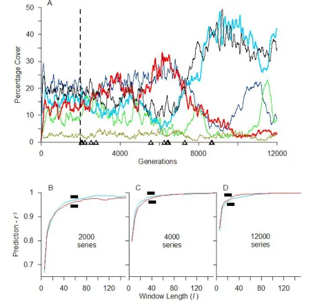
Fig. 5. Effects of a shifting attractor on the CLS of a 20-species system. (A) Temporal dynamics of six of the 20 species. Up to generation 2000, all 20 species coexist and community structure is

approximately constant because “open” recruitment enables recruits of all species to establish (with equal likelihood) on small patches on the landscape cleared by a low level of disturbance (see Methods). At generation 2001, the “open”recruitment is “turned off” and species begin to go locally extinct

Fig. 6. Effects of an invading species (S21 = orange) on the CLS of the 20-species system. (A) Temporal dynamics of three of the 20 species (S9, S14, S20) and the invader (S21). Up to generation 2000, all 20 species coexist and community structure is approximately constant because “open” recruitment enables recruits of all species to establish (with equal likelihood) on small patches on the landscape cleared by a low level of disturbance (see Methods). At generation 2001, the invader is introduced, which is able to overgrow three of the more abundant species, but interactions with all other species are standoffs. The invader attains an equilibrium of ca. 45% cover. (B) and (C) are examples of the landscape at

approximately constant community compositions at 2000 and 7000 generations, respectively. Prediction-r2 spectra are shown for analyses based on series of five maps, each 10 time steps apart, finishing at generation 2000 and 7000 (termed the “2000 series”and “7000 series,” respectively).

shifts in dynamics are evident soon after reducing the growth rate of one species slightly (Fig. 2A) and in shifting the balance of the outcome of interactions between two of the species (Fig. 2B).

The shift in growth rate triggered a change in community structure from approximately equal cover of all species to reduced cover of two species and elevated cover of the other three, including the species (S5) that experienced reduced growth (Fig. 2A). When the outcome of interactions between S1 and S2 shifted from S1 “winning” 100% of encounters to only 60% of encounters, S2 and S4 declined to extinction whereas cover of the remaining three species increased (Fig. 2B). In both cases, a clear shift in the CLS was evident. In the former, the CLS decreased from about 75 to 50 length units (Fig. 3), whereas for the latter model system, the CLS increased from about 75 to nearly 120 length units (Fig. 4).

In the 20-species system, the long-term stable dynamic of 20 coexisting species was disrupted when the steady exogenous supply of propagules to the landscape ceased (Fig. 5A). Immediately after the collapse of open recruitment, several species declined to local extinction. This changed the spatial dynamics between remaining species, ultimately leading to another spate of extinctions. At 10 000 time steps after the cessation of open recruitment, analysis of highly abundant (ca. 40% cover) and relatively rare (<5% cover) species showed that the CLS had reduced from about 55 to about 20 length units (cf. Fig. 5B,C).

Shifts in the length scale of the stable 20-species system following establishment of an invasive species were more subtle and complex (Fig. 6). Before arrival of the invader, several species demonstrated the same length scale of about 55 length units (e.g., Fig. 6D,F), although at least one species indicated a slightly smaller length scale of about 40 length units (Fig. 6H). The invader established and expanded rapidly to dominate ca. 45% of the landscape (Fig. 6A,C), and in this sense, had a major impact on the dynamics of this system. However, although analysis of some species indicated a small (but unambiguous) decrease in the length scale (cf. Fig. 6D,E), within the limits of interpretation of the spectra, analyses based on other species did not indicate a change in the CLS (cf. Fig. 6F,G and 6H,I). Notably, analysis of dynamics of the invasive species indicated a length scale much larger (about 115 length units) than that evident from analysis of the original species (Fig. 6I).

Prediction 3: Two Species Will Indicate Dissimilar CLSs If Their Dynamics Are Largely Independent

In the six-species system (Fig. 7A), encounters between one species (S6) and the other five were always a standoff, and although all species could arise anywhere on the landscape by colonizing bare space created by random disturbance, S6 recruited to these cleared areas at a rate 10 times that of the other five species (see Methods). In these circumstances, the CLS indicated by S6 (about 115 length units) was clearly greater than that indicated by the other five species (about 65 length units) (cf. Fig. 7C,D).

In contrast, in the eight-species system (Fig. 7B), even though a group of five strongly interacting species always realized a standoff in any interaction with the three remaining species (and vice versa), the CLS indicated from analysis of any of the species in the system was similar (Fig. 7E,F).

DISCUSSION

The unifying theme of this collection of papers is scaling thresholds in ecology, and in particular, the application of these quantities to better understand the natural environment and better address the real-world challenges facing ecologists. The primary CLS is defined by a particular scaling threshold (Keeling et al. 1997, Pascual and Levin 1999, Habeeb et al. 2005) that, through recent developments, can now be estimated for real ecological systems (Habeeb et al. 2007, R. Habeeb, C. Johnson, S. Wotherspoon, unpublished manuscript). This scale is a system-level property, and does not necessarily have any relationship with the scales at which any of the many processes that influence a system’s dynamic are manifest. It is a useful quantity because, by definition, it provides an objective means to determine the optimal scale at which to observe the deterministic trend of a system’s dynamic. The results presented here suggest that the utility of the measure might be extended to other important challenges in ecology, namely interpreting temporal change in the structure of ecological communities, and identifying connectivity in the dynamics of different species in complex ecological systems with complex space– time dynamics.

spectra. To date, no attempt has been made to provide a more objective means of identifying the “first point of flattening” of the curve, although there are several possible techniques that might be applied. There are several good reasons for this. First, these curves often show a level of “bumpiness” that has the potential to yield spurious results in applying mathematical analyses of curve structure. Second, there is no logical primacy to select any one of the potential techniques over another, and they will identify different points on the curve. Most importantly, however, small changes in the CLS and a single point-value estimate of the CLS are unlikely to be meaningful in an ecological context. Unless there is a clear shift in the region of flattening of the curve that is discernable by eye, there is a high risk of overinterpretation.

Interpreting Temporal Change in Ecological Systems

The capacity to interpret shifts in community structure is important because changes that reflect a fundamental shift in underlying dynamics may warrant management intervention. If the CLS is to be useful in this context then it must be shown that —providing a system exists in an otherwise stable domain of attraction—the CLS is invariant to even large changes in community structure as a result of deterministic fluctuations. This property is expected on the basis of the theory of non-linear time series analysis and the derivation of the prediction error, i.e., a non-linear oscillating system described by a stationary attractor has a single and constant (primary) CLS (Takens 1981, Keeling et al. 1997, Pascual and Levin 1999). Analysis of the three-species system presented here suggests that the CLS demonstrates this property (Fig. 1), in line with the results of analysis of other model ecologies (Keeling et al. 1997, Pascual and Levin 1999, Habeeb et al. 2005).

It is possible, if unlikely, that the primary length scale of two different attractors is the same. However, if two systems indicate different CLSs then, by definition, they must have different shaped attractors and, therefore, dissimilar underlying dynamics. In keeping with this prediction, when the dynamics of the models presented here were perturbed in some way, in most cases there was a concomitant change in the length scale (Figs. 2–5). For tightly linked systems with strongly interacting

species, even relatively subtle changes in parameters such as the growth rate of a single species or outcome of a particular direct interaction could initiate significant changes in dynamics (Fig. 2). In the 20-species system, halting the endogenous source of recruits resulted in a raft of local extinctions soon afterward and large changes in dynamics, reflected by a shift in the length scale (Fig. 5). This system then experienced a period of relative stability during which a spatially self-organized dynamic was re-established, followed by another set of extinctions and shift in the gross dynamic, with a further corresponding shift in the primary length scale (Fig. 5).

In contrast, depending on which species was analyzed to produce the prediction-r2 spectrum, introduction of a highly invasive species into the 20-species system, which soon proliferated to dominate the landscape, had no detectable effect on the CLS (Fig. 6). At first glance, this may seem to contradict the trends indicated by the other models, but closer inspection reveals several features that illuminate a more complex interpretation. First, the three species chosen arbitrarily for analysis indicate at least two (slightly) dissimilar length scales before arrival of the invader (cf. Fig. 6F,H). This suggests the existence of multiple “sub-communities” whose dynamics are poorly connected (see below), and it is possible that the invader affects one “sub-community” more than another. Further evidence of multiple sub-communities is that one of the three species analyzed does indicate a shift in the CLS after the invader establishes (S9; Fig. 6D,E) whereas the other two do not. This can arise in a 20-species system in which interaction outcomes are chosen at random; some species may have very little influence on others by chance. It is difficult to undertake a more precise analysis because the complexity of linkages in a 20-species competition system where each species potentially competes with every other species for space precludes a precise or systematic analysis of connectivity. Even with as few as 20 species, Darwin’s metaphor of a tangled bank rings true; for every direct interaction between any two species there are about 1.74 ·1016 different possible indirect interactions (Johnson and Seinen 2002).

invader is most clearly observed at a different scale to that of the other species examined. In other words, the dynamic of the invader is not closely coupled with that of the other species examined. This is entirely possible because the invader is able to overgrow only three of the 20 species in the system, and interactions with all other species are a standoff. Once these three species are effectively eliminated from the system as a result of overgrowth by the invader, the invader is maintained only because its interaction with the other species are standoffs, and because its ongoing recruitment is to bare patches that arise randomly and, therefore, independently of the dynamics of any other species (see below). This result emphasizes the need for careful thinking about what is meant by independence or interdependence of dynamics. Even though S21 grows to dominate the landscape, once it attains its quasi-equilibrium density it has very little direct influence on the spatial dynamic of the original 20 species other than by limiting the total amount of space available into which they can grow. Similarly, the 17 original species that manifest standoffs with

S21 have little influence on the dynamics of S21 other than to limit the total amount of space available into which it can grow. This disconnection in dynamics is reflected in the dissimilar length scales. This result serves to emphasize that changes in community structure do not necessarily indicate changes in the dynamical connectivity of many of the component species.

In summary, changes in the CLS of a system, by definition, indicate changes in the underlying dynamics, and the results presented here indicate that in model systems this can arise even with relatively subtle shifts in the attributes of component species. In more complex systems, because the underlying dynamics of different subsets of species might be weakly connected, significant changes in community structure do not invariably mean that all or most species will indicate any shift in the CLS.

These results indicate that we could expect that “phase shifts” from one stable domain of attraction to another in ecological systems as a result of loss of resilience (Scheffer et al. 2001, Folke et al. 2004) are reflected as a change in length scale of the system. Although phase shifts between alternative stable states can be of enormous consequence to ecosystem structure and function and to the humans that depend on them (Folke et al. 2004), obtaining unequivocal evidence of this kind of shift in state is far from trivial (Scheffer et al. 2001) because a shift

in community structure does not necessarily indicate a shift in dynamical state to a different stable configuration. For example, on coral reefs, phase shifts from a coral- to algal-dominated state are, unfortunately, increasingly common and highly problematic (e.g., Done 1992, Hughes 1994, Nystrõm et al. 2000, Mumby et al. 2007). However, declining coral cover on its own or declining coral cover in combination with an increase in algal cover do not necessarily indicate loss of resilience and that the system has shifted to a new stable state dominated by algae. A perturbation such as a hurricane or outbreak of crown-of-thorns starfish might dramatically reduce coral cover and facilitate a flush of algal growth but, in a resilient reef system, the corals will recover and algal cover decline over time (Done 1992, Hughes 1994). However, a similar shift in structure as a result of overfishing of algal grazers (Mumby et al. 2007) could represent an alternative state from which it would be extremely difficult to return to the original coral-dominated state. Given that the dynamics of different stable states of a system are likely to be described by different attractors, then the different states would yield different length scales. Thus, in this way, CLSs could be used as a diagnostic tool to determine whether shifts in structure reflect a shift from one domain of attraction to another, and thus loss of resilience.

This same concept can also be applied to interpreting differences in community structure in space. Comparison of the CLS of ostensibly similar communities in different areas will indicate whether the underlying dynamic is likely to be similar in both areas. This information would be useful, for example, in identifying environmental impact.

Identifying Connectivity among Species in Complex Ecological Systems

It was emphasized in the introduction that ecologists have used many approaches to address the important question of connectivity among species, including several means to measure the strength of interactions between species, chemical tracers to identify trophic pathways, and “natural” and manipulative experiments to identify trophic cascades. The capacity to determine the CLS of natural systems provides another means to assess connectivity. If analysis of the space–time dynamics of two different species on a landscape indicate dissimilar length scales of the system then, by definition, they are describing the dynamics of two different attractors. This suggests that the dynamics of those two species are, to a large extent, independent. Estimating CLSs based on analysis of all species in a community should reveal the number of different groups (i.e., “sub-communities”) of interacting species, within which the dynamics are captured by the same attractor (although I did not attempt this here). Importantly, an assessment of connectivity using CLSs in this way does not require prior knowledge of the nature and strength of interaction between species.

Identifying connectivity in this sense is, of course, qualitative and does not provide any information about the strength of links among species. However, given the complexities of interactions among species in the “tangled bank,” estimations of the CLS provide a relatively straightforward means to identify groups of species that are dynamically coupled, which is useful information.

The examples presented here highlight subtleties to consider in the features that define connectivity. The two models differed in the elements of connectivity that they incorporated. Both the six- and eight-species systems (Fig. 7A,B, respectively) had network topologies in which interactions between some sets of species were always a standoff, i.e., common borders between colonies were stationary

without either species overgrowing the other. In the six-species system, encounters between one species and the other five were always a standoff, whereas in the eight-species system, interactions between three species and the other five were always a standoff. In this sense there was a disconnection in the dynamics of different groups of species in the system; in a standoff, one species is to the other no different than a patch of unsuitable habitat.

However, the two models differ in how occupation of space by the strongly interacting group of five species influenced the amount of the space resource available to the other species in the system. In the six-species system, random disturbances create bare patches on the landscape to which S6 recruits at a higher rate than the other five species. Thus, establishment of S6 at any position on the landscape is possible irrespective of the identity of the species initially occupying that site because disturbance can clear a patch occupied by any species for colonization. The high level of disconnection of the dynamics of S6 with the other five species is indicated clearly by the CLSs (cf. Fig. 7C,D).

The important difference between the eight- and six-species systems is that, in the eight-six-species system, there was no disturbance to clear patches on the landscape. Thus, although all interactions between five of the species and the remaining three were standoffs, their dynamics were ultimately linked by the availability of space on the landscape. Given that most space is fully occupied most of the time, then use of the space resource is a zero-sum game; proliferation of one group of species inevitably impacts on the spatial dynamics of the other despite the disconnection in the network topology. In this circumstance, the length scales indicated by species from the two different groups are identical (cf. Fig. 7E,F).

CONCLUSION

they provide a means of interpreting changes in community structure and identifying loss of resilience and phase shifts, and can be used to identify whether groups of species are dynamically linked.

An important question is whether the behavior of CLSs extracted from models of only three to 20 species is likely to have any resemblance to their behavior in real communities with many more species. It is encouraging that in a real marine fouling community of >50 species, different interacting species with vastly dissimilar life histories, abundances, and taxonomic affinities indicated virtually identical length scales, whereas another species whose dynamics are clearly independent of the others yielded a different length scale (Habeeb, Johnson and Wotherspoon, unpublished manuscript), just as predicted from the results of the models presented here. Given this, and the considerable complexity of the dynamics of models with as few as 20 species, there can be some optimism to expect that the application of CLSs to natural communities will be as useful as their application to model ones. However, this needs further testing empirically.

Although these applications show promise, it is apposite to include a note of caution. Because the capacity to estimate unambiguous length scales is recent, there is much to learn about their properties and how they may be interpreted. For example, the sensitivity of the primary CLS to changes in dynamics, whether the magnitude of changes in the CLS relates in a systematic way to the magnitude of change in the dynamics (however that might be measured), and whether the magnitude of differences in the CLS estimated by analyzing different species on the same landscape is indicative of the magnitude of independence of their dynamics, needs to be determined. Initial indications are that CLSs will not be sensitive to small changes in the space–time dynamics of systems, but arguably this is a desirable property. The CLSs are no panacea, but providing that the tendency to overinterpret spectra is resisted, they are a useful additional tool to address several important issues in applied ecology. If this position is accepted, then there will be a need to ensure that data are obtained that enable this kind of analysis. With advances in several kinds of remote-sensing technology, the availability of suitable space–time data will be increasingly available.

Responses to this article can be read online at:

http://www.ecologyandsociety.org/vol14/iss1/art7/responses/

Acknowledgments:

This work benefited significantly from discussion with Simon Wotherspoon and Rebecca Habeeb and with members of the Modeling and Decision Support Working Group within the Coral Reef Targeted Research Project of the World Bank. The work was supported by an Australian Research Council Discovery Grant. I am also grateful to Robert Washington-Allen for the opportunity to contribute to this collection of papers.

LITERATURE CITED

Bascompte, J., C. J. Melian, and E. Sala. 2005. Interaction strength combinations and the overfishing of a marine food web. Proceedings of

the National Academy of Sciences of the United States of America 102:5443–5447.

Berger, J. O., B. Boukai, and Y. Wang. 1997. Unified frequentist and Bayesian testing of a precise hypothesis (with discussion). Statistical Science 12:133–160.

Borer, E. T., E. W. Seabloom, J. B. Shurin, K. E. Anderson, C. A. Blanchette, B. Broitman, S. D. Cooper, and B. S. Halpern. 2005. What determines the strength of a trophic cascade? Ecology 86:528– 537.

Bruno, J. F., and M. I. O’Connor. 2005. Cascading effects of predator diversity and omnivory in a marine food web. Ecology Letters 8:1048–1056.

Connolly, R. M., D. Gorman, and M. A. Guest. 2005. Movement of carbon among estuarine habitats and its assimilation by invertebrates.

Oecologia 144:684–691.

De Roos, A., E. McCauley, and W. Wilson. 1991. Mobility versus density-limited predator–prey dynamics on different spatial scales. Proceedings

of the Royal Society of London B 246:117–122.

Done, T. J. 1992. Phase shifts in coral reef communities and their ecological significance.

Dunstan, P. K., and C. R. Johnson. 2005. Predicting global dynamics from local interactions: individual-based models predict complex features of marine epibenthic communities. Ecological

Modelling 186:221–233.

Eberhardt, L. L. 2003. What should we do about hypothesis testing? Journal of Wildlife Management 67:241–247.

Fabricius, K. E., and G. De’ath. 2004. Identifying ecological change and its causes: a case study on coral reefs. Ecological Applications 14:1448–1465.

Folke, C., Carpenter, S., Walker, B., Scheffer, M., Elmqvist, T., Gunderson, L., and C. S. Holling. 2004. Regime shifts, resilience, and biodiversity in ecosystem management. Annual Review of Ecology,

Evolution and Systematics. 35: 557–581.

Frank, K. T., B. Petrie, J. S. Choi, and W. C. Leggett. 2005. Trophic cascades in a formerly cod-dominated ecosystem. Science 308:1621–1623.

Greig-Smith, P. 1952. The use of random and contagious quadats in the study of the structure of plant communities. Annals of Botany 16:293–316.

Habeeb, R. 2005. Estimating natural scales of

ecological systems. Dissertation, University of

Tasmania, Hobart, Tasmania, Australia.

Habeeb, R. L., C. R. Johnson, S. Wotherspoon, and P. J. Mumby. 2007. Optimal scales to observe habitat dynamics: a coral reef example. Ecological

Applications 17:641–647.

Habeeb, R. L., J. Trebilco, S. Wotherspoon, and C. R. Johnson. 2005. Determining natural scales of ecological systems. Ecological Monographs 75:467–487.

Hassel, M. P., H. N. Comins, and R. M. May. 1991. Spatial structure and chaos in insect population dynamics. Nature 353:255–258.

Hobbs, N. T., and R. Hilborn. 2006. Alternatives to statistical hypothesis testing in ecology: a guide to self teaching. Ecological Applications 16:5–19.

Hughes, T. P. 1994. Catastrophes, phase shifts, and large-scale degradation of a Caribbean coral reef.

Science 265: 1547–1551.

Hughes, T. P., Bellwood, D. R., Folke, C., Steneck, R. S., and J. Wilson. 2005. New paradigms for supporting the resilience of marine ecosystems.

Trends in Ecology and Evolution 20:380–386.

Johnson, C. R. 1997. Self-organizing in spatial competition systems. Pages 245–263 in N. I. Klomp and I. D. Lunt, editors. Frontiers in Ecology—

Building the Links. Elsevier, Amsterdam, The

Netherlands.

Johnson, C. R., and I. Seinen. 2002. Selection for restraint in competitive ability in spatial competition systems. Proceedings of the Royal Society of

London B 269:655–663.

Johnson, D. H. 1999. The insignificance of hypothesis testing. Journal of Wildlife Management 63:763–772.

Keeling, M. J., I. Mezic, R. Hendry, J. Mcglade, and D. Rand. 1997. Characteristic length scales of spatial models in ecology via fluctuation analysis.

Philosophical Transactions of the Royal Society of London B 352:1589–1601.

Kershaw, K. A. 1957. The use of cover and frequency in the detection of pattern in plant communities. Ecology 38:291–299.

Laska, M. S., and J. T. Wootton. 1998. Theoretical concepts and empirical approaches to measuring interaction strength. Ecology 79:461–476.

Levin, S. A. 1992. The problem of pattern and scale in ecology. Ecology 73:1943–1967.

May, R. M. 2001. Stability and complexity in model ecosystems. Second edition. Monographs in

Population Biology 6. Princeton University Press,

Princeton, New Jersey, USA.

Mumby, P. J., Hastings, A., and H. J. Edwards. 2007. Thresholds and the resilience of Caribbean coral reefs. Nature 450:98–101.

Nowak, M. A., and R. M. May. 1992. Evolutionary games and spatial chaos. Nature 359:826–829.

Nystrõm, M., C. Folke, and F. Moberg. 2000. Coral reef disturbance and resilience in a human-dominated environment. Trends in Ecology and

Pascual, M., and S. A. Levin. 1999. From individuals to population densities: searching for the intermediate scale of nontrivial determinism.

Ecology 80:2225–2236.

Phillips, K. L., G. D. Jackson, and P. D. Nichols. 2003. Temporal variations in the diet of the squid

Moroteuthis ingens at Macquarie Island: stomach

contents and fatty acid analyses. Marine Ecology

Progress Series 256:135–149.

Pimm, S. L. 1992. The balance of nature?

Ecological issues in the conservation of species and communities. University of Chicago Press,

Chicago, Illinois, USA.

Rand, D., and H. Wilson. 1995. Using spatio-temporal chaos and intermediate-scale determinism to quantify spatially extended ecosystems.

Proceedings of the Royal Society of London B

259:111–117.

Ricklefs, R. E. 1990. Ecology. Third edition. W. H. Freeman, New York, New York, USA.

Scheffer, M., S. Carpenter, J. A. Foley, C. Folke, and B. Walker. 2001. Catastrophic shifts in ecosystems. Nature 413:591–596.

Schmitz, O. J., P. A. Hamback, and A. P. Beckerman. 2000. Trophic cascades in terrestrial systems: a review of the effects of carnivore removals on plants. American Naturalist 155:141– 153.

Stewart-Oaten, A., and J. R. Bence. 2001. Temporal and spatial variation in environmental impact assessment. Ecological Monographs 71:305–339.

Takens, F. 1981. Detecting strange attractors in turbulence. Pages 366–381 in D. Rand and L. Young, editors. Dynamical systems and turbulence,

Warwick 1980. Lecture notes in mathematics.

Springer-Verlag, New York, New York, USA.

Tyre, A. J., H. P. Possingham, and C. M. Bull. 1997. Characteristic scales in ecology: fact, fiction or futility. Pages 233–243 in N. I. Klomp and I. D. Lunt, editors. Frontiers in ecology—building the

links. Elsevier, Amsterdam, The Netherlands.

Underwood, A. J. 1994. On beyond BACI: sampling designs that might reliably detect

environmental disturbances. Ecological Applications 4:3–15.

——— 1996. Detection, interpretation, prediction and management of environmental disturbances: some roles for experimental marine ecology.

Journal of Experimental Marine Biology and Ecology 200:1–27.

Watt, A. S. 1947. Pattern and process in the plant community. Journal of Ecology 35:1–22.

Wiens, J. 1989. Spatial scaling in ecology.

Functional Ecology 3:385–397.

Wilson, H. B., and M. J. Keeling. 2000. Spatial scales and low dimensional deterministic dynamics. Pages 209–226 in U. Dieckmann, R. Law, and J. A. J. Metz, editors. The geometry of ecological

interactions: simplifying spatial complexity.

Cambridge University Press, Cambridge, UK.