Convergence of alternating Markov chains

Convergence of alternating Markov chains

G.JONES1&D.L.J.ALEXANDER1

1 _{Institute of Information Sciences & Technology}

Massey University, Palmerston North, New Zealand †

Suppose we have two Markov chains defined on the same state space. What happens if we alternate them? If they both converge to the same stationary distribution, will the chain obtained by alternating them also converge? Consideration of these questions is motivated by the possible use of two different updating schemes for MCMC estimation, when much faster convergence can be achieved by alternating both schemes than by using either singly.

1 Introduction

Suppose A, B are the transition matrices for two Markov chains on the same state space

S which converge to the same stationary distribution. Denoting the space of probability

distributions on S by V, there exists by assumption a unique distribution u∈Vsuch that

A

t n t

v →u and _vtBn _→ut as _{n→ ∞}, for every v_∈V .

Consider now the Markov chain with transition matrix AB. This chain may be derived by repeated alternative application of A followed by B since

(AB) ( A)B

t t

v → v ,

i.e. each AB transition may be regarded as an A transition followed by a B transition. We consider here the convergence properties of this alternating chain, given that each of the component chains converges to the same distribution. Specifically, we investigate whether convergence of AB is assured, and how the rate of convergence of AB relates to the separate rates of convergence of A and B.

2 Motivation

Recent interest in the convergence properties of Markov chains has been stimulated by the current popularity of Markov chain Monte Carlo (MCMC) methods for the estimation of complex statistical models, usually in a Bayesian context. In MCMC a Markov chain is constructed whose stationary distribution is the posterior distribution of the model parameters. For a review of the methodology and its applications see Gilks et al. (1995). Although in most applications the state space is continuous and high-dimensional, the relevant Markov chain theory is often presented in terms of transition matrices on a finite state space, rather than transition kernels, e.g. see Tierney (1994).

This facilitates exposition while still providing useful insight into the essential features of the situation. We shall see that this is particularly true of our present situation.

Rapid convergence to the stationary distribution is a desirable property when using MCMC. It is not uncommon however for convergence to be very slow because of very high correlations between some of the parameters in the model. In such situations it may be necessary for many thousands of iterations to be obtained before valid inferences can be made, and it may even be difficult to assess whether convergence has taken place. Sometimes reparametrization can reduce this problem. An alternative strategy is to find two different MCMC algorithms for the model and to combine them in a hybrid algorithm.

Consider for example the two-component model for errors in chemical assay of Rocke & Lorenzato (1995)

Y = +α βXeη+ε

which relates an assay response Y to chemical concentration X in a linear model subject

to both a multiplicative error η and an additive error ε. Figure 1 shows a typical

calibration dataset for the estimation of cadmium concentrations.

Figure 1: Assay for cadmium concentration by atomic absorption spectrum

Cadmium

Cadmium Concentration (ppb)

Abs

o

r

p

ti

on

0 10 20 30 40

0

2

04

06

08

0

1

0

0

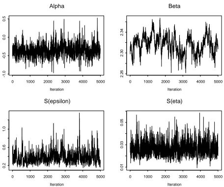
Jones (2004) demonstrates how a naive MCMC analysis using the multiplicative errors as nodes gives very slow convergence because of high correlations between the slope

parameter β and the multiplicative errors at high concentrations. Figure 2 shows a

typical trace of the MCMC output from this algorithm, in which the slow mixing of the

Figure 2: MCMC output for cadmium data

Alpha

Iteration

0 1000 2000 3000 4000 5000

-1 .0 -0 .5 0 .0 0 .5 Beta Iteration

0 1000 2000 3000 4000 5000

2. 2 6 2. 3 0 2. 3 4 S(epsilon) Iteration

0 1000 2000 3000 4000 5000

0. 2 0 .6 1. 0 S(eta) Iteration

0 1000 2000 3000 4000 5000

0. 0 1 0. 0 3 0. 0 5

An alternative algorithm can be derived by taking the additive errors as nodes. We now

find that the α parameter mixes very slowly because of high correlations with the

additive errors at low concentrations. However by alternating each algorithm we get rapid convergence to the stationary distribution.

3 A simple matrix example

Consider the two stochastic matrices .45 .10 .45

A .10 .90 .00

.45 .00 .55

⎛ ⎞ ⎜ ⎟ = ⎜ ⎟ ⎜ ⎟ ⎝ ⎠ and

.45 .45 .10

B .45 .55 .00

.10 .00 .90

⎛ ⎞

⎜ ⎟

= ⎜ ⎟

⎜ ⎟

⎝ ⎠

which have identical eigenvalues λ₁=1,λ₂ =.859,λ₃=.041 and the same stationary

distribution 1 1 1

1 (3 3 3

t

u = ) . The rate of convergence of the Markov chain with

transition matrix A is determined by the "eigenvalue gap" defined as the difference

between the first and second eigenvalues λ λ₁− ₂ =.141, or equivalently by the second

eigenvalue λ₂ =.859. The larger the second eigenvalue, the slower the convergence. To

see this consider the spectral decomposition of A as

1 1 1 2 2 2 3 3 3

A t t

v u v u v u

λ λ λ

= + + t

u

(1)

where are the left-, and u u the right-eigenvectors of A, appropriately

normalized. Because of the orthogonality property of the left- and right-eigenvectors (

1, ,2 3

u u u ₁, ,_{2 3}

t

i j ij

u v =δ ) it follows that

1 1 1 2 2 2 3 3

Since λ₃<λ₂<λ₁=1 it follows that An _{→v u1 1}t as n_{→ ∞} at a rate determined by

2

λ .

However the transition matrix of the alternating chain is

.2925 .2575 .45

AB .4500 .5400 .01

.2575 .2025 .54

⎛ ⎞

⎜ ⎟

= ⎜ ⎟

⎜ ⎟

⎝ ⎠

which has eigenvalues λ₁=1,λ₂ =.369,λ₃ =.003. We would expect much faster

convergence from this chain because of the much smaller second eigenvalue. However

from the MCMC perspective we should properly compare AB with A2 and B2, because

the computational effort in making one AB step would be comparable with that of two

A or B steps. Nevertheless the second eigenvalue of A2 or B2 is so faster

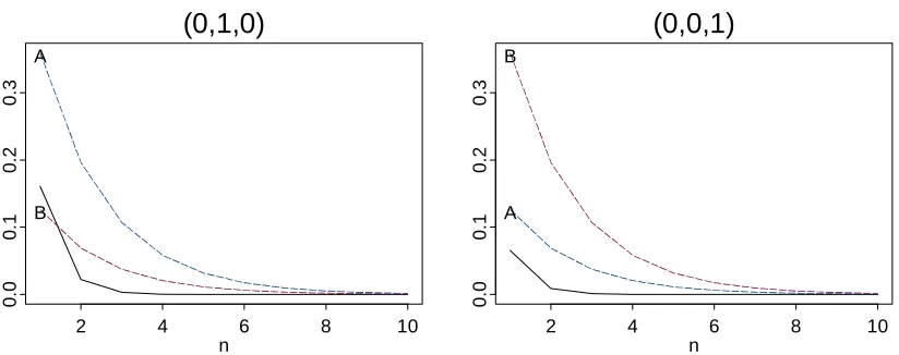
convergence should still be achieved. Figure 3 shows that the alternating chain does indeed converge more quickly to the stationary distribution

2

2 0.738

λ =

1 1 1

3 3 3

( ₎t

1t

than either of the component chains, irrespective of the starting distribution.

(0,1,0)

n

2 4 6 8 10

(0,0,1)

n

2 4 6 8 10

0.

0

0

.1

0.

2

0

.3

A B

Figure 3: Convergence in L2 of A2, B2 (dotted lines) and AB (solid line) from two

alternative starting points

This example works because A and B both have large second eigenvalues whereas that of AB is much smaller. There is however no simple general relationship between these quantities. Moreover the spectral decomposition given in (1) may not be possible in

general because an n×n stochastic matrix may not have n eigenvalues. In the next

section we give some simple results for the general situation.

4 Some general results

Theorem 1: If A and B have the same stationary distribution, so does AB.

Proof: Let u be the stationary distribution. Then _{u AB u B u1}t _{= 1}t _{= .}

0.

0

0

.1

0.

2

0

.3

A

Theorem 2: If A and B converge to the same stationary distribution, AB does not

necessarily converge.

Counterexample: Consider

0.0 1.0 0.0 0.0 0.5 0.5 1.0 0.0 0.0 A

⎛ ⎞

⎜ ⎟

= ⎜_⎜ ⎟_⎟

⎝ ⎠

0.0 0.0 1.0 0.5 0.5 0.0 0.0 1.0 0.0 B

⎛ ⎞

⎜ ⎟

= ⎜_⎜ ⎟_⎟

⎝ ⎠

The eigenvalues of A and B are λ₁=1,λ₂ =.25 .66 ,− i λ₃=.25 .66+ i

and both converge to the stationary distribution 1 1 1

4 2 4

( )t_{. But}

0.50 0.50 0.00 0.25 0.75 0.00 0.00 0.00 1.00 AB

⎛ ⎞

⎜ ⎟

= ⎜ ⎟

⎜ ⎟

⎝ ⎠

is reducible, so does not converge.

Theorem 3: If A and B converge to the same stationary distribution, and B is strictly

positive, then AB converges to the same distribution.

Proof: If B is strictly positive (i.e. every element of B is > 0), it is easy to see that AB is strictly positive - since A is a stochastic matrix each row must have at least one

positive element, with all elements ≥ 0. From Theorem 1 we know that AB has

the same stationary distribution as A and B. Because it is strictly positive it is aperiodic and reducible, so it converges to this distribution.

5 Discussion

The important insight to be gained from the simple matrix examples is that the alternating chain does not necessarily converge. Thus in using a hybrid algorithm for MCMC estimation, care must be taken to ensure convergence. It is possible, as in the counterexample, for the hybrid algorithm to cycle in one part of the state space and not to explore other parts. Theorem 3 gives a sufficient condition for convergence but this is very strong. It may however be useful. In the two-component model example of Section 2 it is easy to show that one of algorithms has a strictly positive transition kernel, since each of the full conditional distributions in the MCMC updating scheme covers the entire range of the respective parameter. Thus convergence of the alternating chain is assured.

References

Gilks W.R, Richardson S. and Speigelhalter D.J (1995). Markov chain Monte Carlo in

practice. Chapman & Hall, London.

Jones G (2004). Markov chain Monte Carlo estimation for the two-component model.

Technometrics, 46:99-107.

Rocke D.M. and Lorenzato S (1977). A two-component model for measurement error in

analytical chemistry. Technometrics, 37:176-184.

Senata E (1979). Coefficients of ergodicity: structure and applications. Adv. Appl.

Prob., 11:576-590.

Tierney L (1994). Markov chains for exploring posterior distributions. Annals of