MoL 2018 12: Advancing the Use of Sparse Knowledge for Qualitative Models and Simulations

(1)

Advancing the Use of Sparse Knowledge for Qualitative

Models and Simulations

MSc Thesis

(Afstudeerscriptie)

written by

Stefania Ionescu

(born December 27th, 1993 in Bucharest, Romania)

under the supervision of dr. Bert Bredeweg and dr. Jaap Kamps, and submitted to the Board of Examiners in partial fulfillment of the requirements

for the degree of

MSc in Logic

at the Universiteit van Amsterdam.

Date of the public defense: Members of the Thesis Committee:

July 20th, 2018 prof. dr. Ronald de Wolf (chair)

(2)

(3)

Abstract

(6)

(7)

Acknowledgments

First and foremost, I would like to thank my supervisors, Dr. Bert Bredeweg and Dr. Jaap Kamps, for their guidance during my first steps into the vast domain of Qualitative Reasoning, and for the patience of answering my questions, even when emails were sent at unreasonable hours. I am very grateful for their time and effort spent in guiding my writing of this thesis, as well as for having faith in good final results even when progress was really slow.

Lots of thanks also to the other members of the committee, Prof. Ronald de Wolf, Dr. Kaspar Beelen, Dr. Anders Bouwer, and Dr. Marijn Koolen who had the patience of going through pages of sometimes impenetrable mathematical notation. A huge thanks to Dr. Wielemaker for helping with all the SWIProlog related questions, and especially for his clarifications on the working of the profiler which was extremely valuable in the early phase of our work. Next, I would also like to thank Prof. Benedikt L¨owe for the mentoring done throughout my two years in the Master of Logic, and to Dr. Thomas Forster for guiding my steps into taking this program.

(8)

(9)

Chapter 1 Introduction

Since there is an enormous gap between the infinite complexity of the world and our finite knowledge of it, people react to the environment using their internal representations, which are based on incomplete information (Kuipers, 1994). This incomplete information is usually expressed qualitatively, by the relative differ-ence between quantities, rather then quantitatively, by giving in exact numerical values. For example, two people discussing future weather conditions would say “the temperature in Amsterdam will be slightly higher than the one in Utrecht”, rather than “the temperature in Amsterdam will be equal to the one in Utrecht plus one degree”.

Qualitative Reasoning (QR), which is a field of Artificial Intelligence, investi-gates how this type of reasoning can be automated (Van Harmelen et al., 2008). The aim of this field is to develop the means for creating a model that captures the available qualitative information (system structure, assumptions, conditions etc.), and that can infer possible outcomes through simulation. The need for rea-soning with incomplete knowledge and for human-machine interaction motivates QR applications in a variety of subjects such as physics (De Kleer, 1990), ecology (Bredeweg and Salles, 2009), engineering (Abbott et al., 1988), and robotics (Pin et al., 1992). Lastly, it is very useful in education, as it gives a natural learning environment for students in science, enabling them to formalise their knowledge into models and use it through scenario simulations (Bredeweg and Forbus, 2003). The focus of this thesis is on addressing the resolution problem, which is one of the three main QR problems according to Weld and De Kleer (2013). In short, since usually not all the necessary information is possessed, there is a need for reasoning techniques that work even under partial knowledge. This means our focus is on addressing the following research question:

How can we maximise the information inferable from sparse knowledge in process-oriented qualitative reasoning?

(10)

cita-tions), but tailored to the needs of addressing our research question focussing on simulation rather than modelling. This axiomatisation is then used both to point out incoherences and to find procedures for early identification of incompatible system behaviour developments. The time analysis of these procedures is mostly done theoretically. Occasionally, we look at some particular examples to investi-gate practical benefits of our algorithms. This case analysis is done by running simulations in Garp3 (Bredeweg et al., 2009), which is a workbench based on an executable language that allows users to construct, simulate, and analyse models based on qualitative knowledge.

This thesis is structured around four main chapters, each addressing a spe-cific question and contributing towards answering our main research question. Chapter 2 investigates how the earlier formalisations of process-oriented quali-tative reasoning can be adapted to allow for theoretical analysis of simulations. Consequently, this chapter brings three main contributions. First, it provides a brief literature review of process-oriented QR. Second, it builds the clarity and the vocabulary needed to theoretically discuss qualitative simulations by devel-oping a partial axiomatisation. This is mostly based on the earlier formalisations of Bredeweg et al. (2009), Liem (2013), and Linnebank (2004), but focusses on defining the concepts needed in simulations and on providing clear notations and definitions, similar to the work of Weld (1988). Third, to illustrate those defi-nitions, a novel model from the field of Auction Theory is introduced. Fourth, a large simulation example (Kansou et al., 2017) is used for further clarifying the definitions and the simulation steps, and for a practical illustration of the problems associated with sparse knowledge.

In Chapter 3, the question addressed is of whether, because of sparse knowl-edge usage, principles of consistency are violated by the current qualitative sim-ulation approach. First, this chapter underpins three types of incoherent be-haviours that could be predicted by the previously axiomatised simulation ap-proach. These violate either (a) model consistency, i.e. each state must be in accordance with the model, both in point of dependencies and relations, (b)path consistency, i.e. each possible sequence of events predicted should be coherent, and in particular should not contain contradictory assumptions or misrepresent extrema, or (c) inexplicit inequality consistency, i.e. the simulation result should also be in accordance with the inequalities that are not explicitly stated. Second, it finds solutions for solving these particular types of incoherences.

(11)

3

to solve this problem in polynomial time. Third, a faster algorithm for COMB, which is better for practical use, is provided.

Chapter 5 investigates how the solutions for the general problem presented in the previous chapter can be adapted for efficiently using the sparse knowledge in qualitative simulations. First, it finds that, in the case of non-changing models, there is a reduction from COMB to the problem of finding plausible simultane-ous next-state developments of systems (ELIG). Second, it adapts the previous solution to work under changing models. Third, the benefits of these solutions are illustrated by returning to the two examples from the second chapter.

(12)

(13)

Chapter 2 Modelling and Simulation in the

Context of Qualitative Reasoning

This chapter aims to provide a clear understanding of process-oriented Qualitative Reasoning, which is necessary for answering the research question posed in the introduction. To achieve this, first, a partial axiomatisation for process modelling and simulation is developed. Second, two examples of simulations are then used with the double purpose of illustrating the concepts introduced in the earlier parts of the chapter, and of hinting potential problems resulting from sparse knowledge usage.

2.1 Qualitative Modelling and Simulation

As mentioned in the introduction, this thesis considers an executable language with logical constraints. Therefore, after modelling a system, the user can de-scribe a situation (by means of an initial scenario) and run the model to analyse the possible qualitative developments. Hence, the process can be broken into three phases, namely: understanding the model language, introduced in Sub-section 2.1.1, describing a state in the world, discussed in Subsection 2.1.2 and simulating the model, presented in Subsection 2.1.3. This section is based on the previous formalisations of Bredeweg et al. (2009), Liem (2013), and Weld (1988).

2.1.1 Modelling Language

(14)

the information contained within the model. Moreover, an algorithm can now interpret the information and use it to produce predictions (i.e. run simulations). Therefore, one needs first to understand a standardised language in order to construct models. In this thesis, we build upon the language proposed by Bredeweg et al. (2009). This is also used in Garp3, which will be the workbench used for running examples. There are a multitude of ingredients used to construct this language, and this subsection presents the structural ones.

Entities are the basic structural compounds of the system which do not change during the simulation phase. Formally, we define an entity as a finite set of quantities, E ={Q1, ..., Qn}. Quantities are the changeable features of entities.

For instance, the quantity “size” of the entity “population” might change over time. Similarly, the quantity “bid” of an entity “bidder” has different values throughout a simulation. At any given time, a quantity has also the tendency to either increase, remain steady or decrease. This tendency is given by the value of the derivative of a quantity at that given moment.

Hence, a quantity Q is defined as a variable, which has another associated variable named (first order) derivative, denoted by dQ. Moreover, if Q is a set of quantities, then the set of associated derivatives is denote by dQ, i.e. dQ = {dQ|Q ∈ Q}. A parameter is defined inductively; any quantity is a parameter, and so are the derivatives of any parameter. For practical reasons, not all order derivatives are considered. In general, for a given set of quantities, the associated parameters are only these quantities together with their first order derivatives, that is PQ :=Q ∪dQ. Notice that this is different from the usual definition of a

parameter (Weld and De Kleer, 2013).

The qualitative values that parameters can take are described by landmarks

and intervals. For instance, a bid could be “zero”, “plus”, or “maximum”, where “zero” and “maximum” are points (i.e. landmarks) while “plus” is an interval. The meanings associated with these are that the bid stands at zero, a positive value, or the maximum amount the bidder is willing to offer, respectively. For-mally, landmarks are considered constants that can be partially ordered by the strict relation <. Two landmarks lu, lv within the set L of all landmarks are

considered consecutive if lu < lv and there is no lt∈ L such that lu < lt < lv. As

always, given a set of landmarks L, a minimal landmark is an l1 such that there

is no l0 ∈L with l0 < l1 (and similarly for the maximal).

An interval is also a constant which is associated either with two consecutive landmarks or with a minimal or maximal landmark. So, for the consecutive landmarkslu < lv, the associated interval will beiu,v. If l1 is minimal, theni0,1 is

its associated interval, while if lu is maximal it will have iu,u+1 as an associated

interval. The partial order < also extends over intervals, so lu < iu,v < lv.

However, the relation is not strict over intervals, as iu,v < iu,v is valid. The

(15)

2.1. Qualitative Modelling and Simulation 7

being almost at maximum.

A given quantity can take different values depending on its nature. Therefore, while modelling the system, the user needs to specify the qualitative values that each quantity can take. So, for each quantity, there is an associated magnitude space formed of landmarks and intervals, in which its value can vary. The land-mark space associated with a quantityQ is defined as a set of landmarks totally ordered by <, LQ = {l1 < l2 < ... < lm} that quantity Q can take, while the

interval space ofQis the set of intervals associated with these landmarks, that is

IQ ={i1,2, i2,3, ..., im−1,m} possibly together with one or both of i0,1 and im,m+1.

The magnitude space of Qis hence the set of landmark and interval spaces of Q, i.e. MQ =LQ∪IQ.

Intuitively, the value of a derivative of a parameter P shows the tendency of change for that parameter. So, a derivative should be either negative, indicating thatP is decreasing, zero, indicating that it is stable, or positive, indicating that it is increasing. Hence, for any parameter P, LdP = {0}, IdP = {−,+}, and

MdP ={−<0<+}.

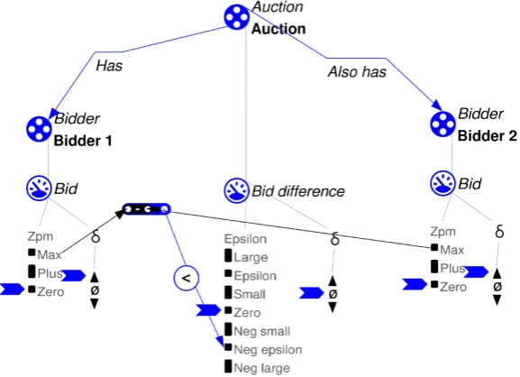
The model for a bidder, which is depicted in Figure 2.1, illustrates the concepts defined above (see Section 2.2 for details and motivation on the auction model). The entity Bidder has two associated quantities, namely Bid and To absolute. Using the notation, Bidder ={Bid,To absolute}. The landmarks for the quan-tity Bid are 0 and Max, and there is only one interval, namelyPlus. Hence, the landmark space is LBid = {0,Max}, the interval space is IBid ={Plus}, and the magnitude space is MBid = {0,Plus,Max}. As usual, the magnitude space for

the derivative isMdBid ={−,0,+}.

Note however that the magnitudes are not necessarily equal between quanti-ties, even though they have the same name. If two quantities Bidder1,Bidder2

haveMax in their magnitudes space, formally they have the two associated land-marks MaxBidder1 and MaxBidder2, which in general might not be equal. However,

[image:15.595.216.378.550.682.2]

to simplify notation, the indices are sometimes dropped.

Figure 2.1: A model fragment for the English Auction model.

(16)

composing it, but rather from the interrelated nature of those elements. Usually, a change in one quantity determines a change in another, which in turn might have various effects on other quantities. For example, if a bidder is not the absolute winner, that is it the value of itsTo absolute quantity is positive, this determines an increase of its bid. This is modelled using causal ingredients, which are of three types:

• Proportionality (which can be either positive or negative) models a corre-lation between the tendencies of two quantities. An example is the pro-portionality between the size and the number of births of a population: if the first increases, this will determine an increase in the second. More pre-cisely, if Q1 is positively proportionally influenced by Q2, Q1 has no other

dependencies, and Q2 is increasing, thenQ1 should also be increasing.

More formally, the two types of proportionality are denoted byP+ orP−, and each of them is an antisymmetric binary relation onQ.

• Influence (which can be positive or negative) models the dependency be-tween the magnitude of a quantity and the tendency of another. To take an example, the number of deaths negatively influences the size of a population as, if the number of deaths is positive, and there are no births or immigra-tion, then the size of the population should decrease. More precisely, if Q1

is positively (directly) influenced byQ2,Q1 has no other dependencies, and Q2 is positive, thenQ1 should also be increasing.

Formally, the two types of influences are denoted byI+ or I−, and each of them is an antisymmetric binary relation on Q.

We also say that a dependency is either an influence or a proportionality relation.

• Correspondence, which can be directed or undirected, shows co-appearing magnitudes. For example, in an auction with two bidders, a zero difference between the two bids means that the two bidders are not the absolute winners, so their To absolute quantities should be Plus. Hence, a bidding difference of zero unidirectionally corresponds to a To absolute value of

Plus.

Formally, the directed (value) correspondence setC is a binary relation on PQ× ∪P∈PQMP. More precisely,

C ⊆ {((P1, v1),(P2, v2))|Pi ∈ PQ, vi ∈MPi, P1 6=P2}.

(17)

Additionally, the undirected correspondence is symmetric. However, since the undirected correspondence can be expressed in terms of directed corre-spondences we will only use the latter, to which we will refer to simply as correspondences.

With the elements presented above, one has the needed language to construct a model. The inequalities extended to quantities, as well as the option of mod-elling by fragments, are also useful, but will be discussed in the next subsection. However, on its own, this language is not sufficient as, in order to use it, one should be able to provide a description of the current state of the world, as well as to run it in order to predict possible future developments.

2.1.2 World Description

Up to this point, the language for encoding the general information that remains true throughout any simulation was presented. That is only the information that does not depend on any particular value. However, in order to make the model useful, one should be able to supply information about the state of the world at a particular time. This means providing details about the magnitudes of the quantities used and their derivatives, the relations between different quantities, etc. In this subsection, we build the vocabulary used to provide the model with a (partial) description of its state at a particular time.

Firstly, (in)equalities are used to compare certain ingredients. These are bi-nary relations R ∈ {<,≤,=,≥, >}, which can appear between two quantities, landmarks or derivatives, a quantity and a landmark, or a derivative and zero. More precisely, for a given set of quantitiesQ, the elements of the relationsR are of the form:

• (Q1, Q2), for Q1, Q2 ∈ Q, i.e. comparing two quantities;

• (Q, l), forl ∈LQ, i.e. comparing a quantity and a landmark;

• (l, l0), forl, l0 ∈LQ, Q∈ Q, i.e. comparing two landmarks;

• (dQ1, dQ2), forQ1, Q2 ∈ Q, i.e. comparing two derivatives;

• (dQ,0), for Q∈ Q, i.e. comparing a derivative and zero.

This is also extended to inequalities on terms, that is on expressions obtained from parameters together with arithmetic operators.

(18)

In addition, one should also be able to specify qualitative values for different ingredients in order to compare them. That is, if at a certain moment the bid of the first bidder is 0, and a prediction of possible future developments from that state is desired, one should be able to specify this value. A specification of one or more such values will be referred to as an assertion. Formally, this is defined as follows:

• A magnitude assertion for the set of quantities Q is a (partial) function

mag :Q → ∪Q∈QMQ, such that mag(Q)∈ MQ for all Q∈ Q and mag(Q)

defined. Hence, a magnitude assertion for Q is a function that gives to (some) quantities in Qsome magnitude within their associated magnitude space.

• A derivative assertion for the set of quantities Q is a (partial) function

der:dQ → {−,0,+}.

• Aqualitative value assertionfor the set of quantitiesQis a (partial) function

val :Q∪dQ → ∪Q∈QMQ∪{−,0,+}such thatvalm :=val|Q is a magnitude

assertion, andvald:=val|dQ is a derivative assertion.

As an example, in Figure 2.2 there is a magnitude assertion for the set of quantities Q={Bid1,Bid2,Bid difference} is a total function, such that:

• mag(Bid1) =mag(Bid2) = mag(Bid difference) = 0,

• mag(dBid difference) = 0, and

• mag(dBid1) =mag(dBid2) = +.

Moreover, since there are no derivative specifications, the qualitative value asser-tion is the same as the magnitude asserasser-tion.

This gives all the elements to define a scenario, that is a partial qualitative description of a situation. A scenario captures information about the qualitative values and the relations between different ingredients of the model. Moreover, the two elements of the scenario must be consistent with each other. For example, if two quantities are equal, and they also have asserted values, then their values should not be specified as being unequal.

An example of a scenario, realised using Garp3, is pictured in Figure 2.2. This scenario presents an auction with two bidders, each of them currently bid-ding zero, but with a tendency to increase the bid. In addition, the difference between the two bidders is currently zero and stable. Finally, the second bidder has a higher valuation than the first one, meaning that they are willing to bid (significantly) more.

Formally, a scenario s is a tuple hE,val, <,≤,=i, where E is a set of entities,

(19)

[image:19.595.154.443.118.327.2]

Figure 2.2: English Auction with two bidders: initial scenario

R ∈ {<,≤,=}, then the relation between P1 and P2, if specified, should be

val(P1) R val(P2), where P1, P2 are parameters in E, formally inP∪E∈EE.

Another useful concept is that of model fragments (MF), used to describe how parts of the system behave under certain conditions. One such example was already mentioned in Figure 2.1. The conditions are shown in red, and the consequences in blue. As a result, the model fragment reads as follows: if there is an entityBidder with quantitiesBid andTo absolute, such thatBid is at a value smaller than Max, then the To absolute quantity positively influences the Bid. Notice that the same model fragment can be used multiple times. For example, if there are two bidders respecting the conditions of this model fragment, as it is the case in Figure 2.2, then the model fragment would apply for both.

An active model fragment for a given scenario, is a model fragment that has the conditions satisfied by that scenario. In order to provide a formal definition for model fragments, a classification of the different types of ingredients is needed. The behaviour ingredients of a scenario are the relations and the value as-sertion function. That is, the behaviour ingredients of s = hE,val, <,≤,=i are

val, <,≤,=. The structural ingredients of a scenario are the set of its entities (which also contains information about quantities), together with agents, config-urations, attributes, and assumptions. The last four types are beyond the scope of this thesis, so we will not insist on these. In general, the conditionals of a scenario are its structural and behavioural ingredients.

(20)

ingredients together with (in)equality relations.

Therefore, for every state there are associated proportionality, influence and correspondence relations, plus possible (in)equality restrictions, that are given by the MF function. Those will be referred to as the set ofactive causal ingredients, which, for a scenario s, is given by S

Co⊆Condsmf(Co).

So, in this section, an axiomatisation for a state description was provided. In addition, model fragments were used to account for case distinctive behaviours of the system. The focus of the next section is on running a scenario in the context of a given model fragment function.

2.1.3 Model Simulation

Having constructed a model, and presented it with an associated scenario, it is now time to run the model with the scenario in order to predict possible system behaviours. This is referred to as a simulation. Throughout this subsection, the focus will be on providing the vocabulary for describing the simulation of a model fragment function and a scenario.

To begin with, a state represents a complete version of a scenario. Differently from a scenario, a state has known qualitative values for all the magnitudes of quantities. More precisely, a state s is a scenario for which the magnitude assertion is total, i.e. the qualitative value assertion restricted on quantities (valm) is a total function. Furthermore, a state s extends a scenario s0 if all the

elements of s are supersets of the respective ones in s0. If the scenario is under-specified, it can have more than one state extension. In that case the scenario is called ambiguous.

In order to capture the dynamic nature of a system, states must be able evolve into new ones. The way a state changes is byterminating the current one. Hence, asimple termination is defined as a pair capturing a cause and a set of resulting changes. So, a simple termination for a statesis a pair (c,Re), wherecis a cause, and Re is a set of results. Moreover, the tuple needs to satisfy the termination validity criteria which will be defined later. The set of results is a collection of relations on the parameters of s, while the different types of causes are defined below.

A cause cof a termination for a state s=hE,val, <,≤,=iis a pair that gives the type of change (i.e. a constant from Table 2.1) and a quantity (or a pair of quantities) from∪E∈EE, i.e. c= (cause name, Q), for some Q in∪E∈E E. Table

2.1 presents the causes grouped into three possible categories. Formally, there are four categories, as there are also exogenous terminations on derivatives (Bredeweg et al., 2009), but these necessitate additional constraints, and are outside the scope of this thesis. In additon, for the derivative and inequality causes, there are also assumed versions of the constants, e.g. (assumed derivative stable to down, Q).

(21)

Class of causes Type of cause

Value causes (to point above, Q) (to point below, Q) (to interval above, Q)* (to interval below, Q)*

Derivative causes (derivative stable to down, Q)* (derivative stable to up, Q)* (derivative down to stable, Q) (derivative up to stable, Q) Inequality causes (from equal to greater,(Q1, Q2))*

(from equal to smaller,(Q1, Q2))*

(from smaller to equal,(Q1, Q2))

(from greater to equal,(Q1, Q2))

(from smaller or equal to smaller,(Q1, Q2))∗

(from smaller or equal to equal,(Q1, Q2))

(from smaller or equal to greater,(Q1, Q2))∗ (from greater or equal to greater,(Q1, Q2))∗

(from greater or equal to equal,(Q1, Q2))

[image:21.595.113.503.116.421.2]

(from greater or equal to smaller,(Q1, Q2))∗

Table 2.1: Types of causes

s = hE,val, <,≤,=i, t needs to satisfy the termination validity criteria. This means that only certain pairs of causes and results are valid. Moreover, these are valid for the state sonly when a certain set of conditions (constraints) of sis valid. The condition function ofs, denoted bycond, is a function from the set of simple terminations to the power set of constraints ofs. Hence,cond(t) is the set of constraints for the termination t. Table 2.2 outlines the termination validity criteria. This is based on the work of Linnebank (2004).

Not all terminations have the same level of priority, as some happen before others. The set of terminations is therefore divided into two parts, namely imme-diate terminations, which are from a point or from equality, i.e. the ones marked with * in Table 2.1, and non-immediate terminations, which are to a point or to equality. Hence, the set of simple terminations Ts is the disjoint union of the

set of immediate terminationsIs and the set of non-immediate terminations Ns.

That is,Ts =Is∪N˙ s.

(22)

Cause type Elements of cond(t) Elements of re-sults set

(to point above, Q) val(Q) =iu,u+1, foriu,u+1 ∈IQ

val(dQ) = +

val(Q) =lu+1

val(dQ)≥0 (to point below, Q) val(Q) =iu,u+1, foriu,u+1 ∈IQ

val(dQ) =−

val(Q) =lu

val(dQ)≤0 (to interval above, Q) val(Q) =lu, forlu ∈LQ

val(dQ) = +

val(Q) =iu,u+1

val(dQ)≥0 (to interval below, Q) val(Q) =lu+1, forlu+1 ∈LQ

val(dQ) =−

val(Q) =iu,u+1

val(dQ)≤0 (derivative stable to

down, Q)

val(dQ) = 0

val(ddQ) = −*

val(dQ) =−

val(ddQ)≤0* (derivative stable to

up, Q)

val(dQ) = 0

val(ddQ) = +*

val(dQ) = +

val(ddQ)≥0* (derivative up to

stable, Q)

val(dQ) = +

val(ddQ) = −*

val(dQ) = 0

val(ddQ)≤0* (derivative down to

stable, Q)

val(dQ) =−

val(ddQ) = +*

val(dQ) = 0

val(ddQ)≥0* (from equal to greater,

(Q1, Q2))

Q1 =Q2 dQ1 > dQ2*

Q1 > Q2 dQ1 ≥dQ2*

(from equal to smaller,

(Q1, Q2))

Q1 =Q2 dQ1 < dQ2*

Q1 < Q2 dQ1 ≤dQ2*

(from smaller to equal,

(Q1, Q2))

Q1 < Q2 dQ1 > dQ2*

Q1 =Q2 dQ1 ≥dQ2*

(from greater to equal,

(Q1, Q2))

Q1 > Q2 dQ1 < dQ2

[image:22.595.94.499.110.561.2]

Q1 =Q2 dQ1 ≤dQ2*

Table 2.2: Termination validity criteria. Note that the inequality transitions from a weak constraint to a strong one were omitted, but these are similar to the mentioned ones. In addition, if the constraints marked with star do not appear explicitly, but could be added while maintaining consistency of the state, then the cause is assumed.

(23)

it is composed by non-immediate terminations. Formally,

T ⊆

(

Is, if Is 6=∅

Ns, otherwise

,

whereIs is the set of immediate terminations ofs,Ns is the set of non-immediate

ones, and T is a compound termination. This rule of prioritising immediate terminations will be referred to as the epsilon ordering rule.

The set of compound terminations of s is denoted by Ts. The set of causes

of the compound termination T is the set of causes that belong to the simple terminations within T, that is {c|(c,Re)∈ T}. Similarly, the results of T is the union of the result sets of the simple terminations, i.e. ∪(c,Re)∈TRe. Moreover,

the condition function naturally extends over compound terminations by letting

cond(T) =∪t∈Tcond(t).

The physical world is continuous, in the sense that there are no jumps in tendencies between consecutive states of the same system. So, the continuity criterion states that the tendency of a quantity cannot jump from the positive to the negative interval or vice-versa without first passing through zero. Another way of saying this is that a pair of states (s1, s2) satisfies the continuity criterion iff for every parameter P appearing resulting from the entity spaces of the two states the following holds:

• if val1(dP) =−, then val2(dP)≤0

• if val1(dP) = +, then val2(dP)≥0

At this point a state and a compound termination can produce a new state by implementing the resulting changes, captured by the termination, into the old state. A transition scenario from state s with the compound termination T is then defined as the scenario s0 obtained from s by changing with the results in

T, that is withReT =∪(c,Re)∈TRe.

However, simply making the changes within a state does not guarantee the consistency of the state, as it is not necessarily in accordance with it active causal ingredients. Therefore, we say that a state s = hE,val, <,≤,=i with its active causal ingredients P+, P−, I+, I−, C is stable if:

• There is an influence balance. This happens when the qualitative value assertionval is plausible with the influence relation of s. Formally, that is when for every Q∈ ∪E∈EE, the relation

dQ= X

(Q1,Q)∈I+

f1(Q1)−

X

(Q2,Q)∈I−

f2(Q2),

where the functionsfi are strictly increasing and with zero as a fixed point,

(24)

• There is a proportionality balance. Similarly, this happens when the quali-tative value assertionval is plausible with the proportionality relation ofs. Formally, that is when for every Q∈ ∪E∈EE, the relation

dQ= X

(Q1,Q)∈P+

g(dQ1)−

X

(Q2,Q)∈P−

g(dQ2).

where the functionsgi are strictly increasing and with zero as a fixed point,

holds. Notice that in this case, because of the possible values of the deriva-tives, the relation is equivalent with val(dQ) = P

(Q1,Q)∈P+val(dQ1) −

P

(Q2,Q)∈P−val(dQ2).

• There is a correspondence fit. This happens when the qualitative value as-sertionval is plausible with the correspondence relation ofs. Formally, that is when for everyP1, P2 ∈ ∪E∈EEandvi ∈Mi, such that ((P1, v1),(P2, v2))∈ C, ifval(P1) = v1, then val(P2) = v2.

Notice that the influence and proportionality balances are separate, and not mixed. The reason for this is that in qualitative reasoning, the dependencies are interpreted as causalities, so a quantity cannot have both incoming influences and proportionalities.

There are now all the components needed to define the possible developments of a current state. A successor of a state s is a continuous and stable state

s0, extending the transition scenario of s and some compound termination T. The change between the successive states s and s0 is captured by a transition. Hence, a transition is formally defined as a pair of successor states (s, s0). Now there is a visual representation of the system’s development by the states and the transitions between them. This is in the form of a state graph (or behaviour graph), which is a directed graph G = (V, E) where V is a set of states and E

is the set of transitions between them. Moreover, any behaviour graph must be maximal, in the sense that there is no state in V with a successor outside V. A path in this state graph, which shows a possible development of the system, is referred to as atrack. Examples for those are discussed in the next section.

This finalises our axiomatisation of the system. As mentioned in the intro-duction of this section, this is only a partial one meant to bring the conceptual clarity needed for investigating the research question. Throughout this section, the formal definitions were illustrated using examples from an English Auction model. These example will be discussed in the next section.

2.2 Continuous English Auction with Two

Bid-ders from a Qualitative Perspective

(25)

2.2. Continuous English Auction in QR 17

the first subsection discusses the English Auction, the second one the modelling, and the last one, the simulation.

2.2.1 Continuous English Auction

During a classical English Auction, an item is presented to people in the room, and the ones interested bid for this item. Each person has a valuation, that is a maximum value that they are prepared to bid. During the bidding, one person starts with an offer. If anybody is willing to offer more, they can challenge the highest current bid by offering a higher amount. The auction stops when nobody wants to bid over the highest offer. The item is usually indivisible, so there can only be one winner (McAfee and McMillan, 1987).

This system is obviously not continuous. However, for theoretical analysis in Auction Theory, the continuous version is used. According to that, the bidders increase their offer in a continuous manner, and the winner is the person that offers more than any other one by at least some epsilon (an arbitrarily small con-stant). This version is similar to the ascending bid or Japanese Auction (Milgrom and Weber, 1982), where the interested people stay in a room where an initial price is displayed. The price increases continuously, and the bidders that are not interested in purchasing the item at that price exit the room. The winner is the last bidder remaining in the room.

For clarity, this section aims at modelling the continuous version of the English Auction for two bidders only, but the same principles can be used for larger num-bers of bidders. To achieve this aim, the model fragments need to be constructed based on entities. This is done in the Subsection 2.2.2.

2.2.2 Qualitative Model

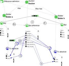
Having described what a Continuous English Auction is, this subsection presents the model fragments used for its qualitative modelling. Figure 2.1, already showed one such model fragment. This encodes an obvious strategy for a bidder, namely that if their bid is not maximum, then the difference they have until becoming the absolute winner positively influences their bid. Another model fragment, shown in Figure 2.3, says that once at the maximum value, the bid stagnates, i.e. one cannot bid over their valuation. The fragment in Figure 2.4 ensures that the bidding difference is indeed the first bid minus the second one, that is Bid difference = Bid a −Bid b. There are also proportionality relations: a positive one fromBid a toBid difference, as an increase in the first bid produces an increase of the difference, and a negative one fromBid b toBid difference, as if the former increases the latter would decrease. In addition, the Epsilon and

(26)

[image:26.595.154.442.281.486.2]

Figure 2.3: English Auction with two bidders: model fragment for the strategy according to which bidders do not bid over their valuation.

Figure 2.4: English Auction with two bidders: model fragment for the behaviour of Bid difference.

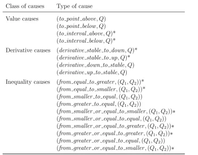
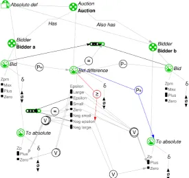
The only quantities not covered by the previously introduced model fragments are theTo absolutequantities of the two bidders. To do this, the model fragment from Figure 2.4, is extended to the one in Figure 2.5, which shows the corre-spondences for theTo absolute quantities. A bidder is the absolute winner if the difference between them and any other bidder is at least epsilon. For the case of two bidders, this means that To absoluteBiddera = 0 iff Bid difference ≥Epsilon,

and To absoluteBidderb = 0 iff Bid difference ≤ Neg epsilon. This is precisely

what is encoded by the value correspondences in the model fragment. In addition, wheneverTo absolute has a non-zero value, it is proportionally influenced by the

Bid difference ≥ Epsilon. In other words, whenever Bid difference ≤ Epsilon

this negatively proportionally influences To absoluteBid a, see Figure 2.6, and

whenever Bid difference ≥ Neg epsilon this positively proportionally influences

(27)

[image:27.595.160.434.160.421.2]

wheneverBid difference isLarge orEpsilonand otherwise it increases if and only if Bid difference is decreasing.

Figure 2.5: English Auction with two bidders: model fragment showing the cor-respondences from the Bid difference quantity to theTo absolute quantities.

This finalises the building of the model for the English Auction. It was done via six model fragments that encode the obvious strategies of the bidders, i.e. “do not bid over valuation”, “if the bid did not reach the valuation, increase bid iff not the absolute winner”, as well as the behaviour for the other quantities, i.e. theBid difference which is the difference between the two bids, and the two

To absolute quantities. In the next subsection the simulation is discussed.

2.2.3 Example of a Simulation

This section presents the simulation for the scenario in Figure 2.2. Remember that according to that scenario, the maximum ofBid1 is lower than the maximum

of Bid2 by a non-negligible amount, that is an amount greater than Epsilon. In

addition, the two bids are currently at zero, as is their difference.

(28)

[image:28.595.159.435.113.375.2]

Figure 2.6: English Auction with two bidders: model fragment showing how

Bid difference influences the To absolute of Bid a.

Bid difference, and second order derivatives are unknown, there are also assumed derivative terminations for this quantity. So the other two simple terminations are (assumed derivative stable to up,Bid difference), and (assumed derivative stable to down,Bid difference). The compound terminations in Figure 2.8c are obtained by combining the simple ones. Since the two value terminations are immediate and non-assumed, by epsilon ordering, they should always co-appear. Moreover, the two assumed terminations are contradictory, so they cannot co-occur. Therefore, the three compound terminations that may produce successor states are obtained from the two value terminations together with one or no assumed derivative change. Each of these gives a successor for 1.

To continue this example, consider state 2. In this state both bids are, ac-cording to the valuation, Plus and have a positive derivative. Moreover, the

Bid difference is 0 and decreasing. According to the model fragments in figures 2.5, 2.6, and 2.7, both To absolute quantities are Plus, the one corresponding to a is increasing, while the one corresponding to b is decreasing. This state has five simple terminations, as shown in Figure 2.9a, but only one of those, namely (to interval below,Bid difference) is an immediate termination, so this forms alone the only compound termination, see Figure 2.9b. Consequently, only one successor for state 2 exists, as shown in Figure 2.9c.

(29)

Figure 2.7: English Auction with two bidders: model fragment showing how

Bid difference influences the To absolute of Bid b.

(a) The extension of the initial scenario.

(b) The simple ter-minations.

(c) The compound terminations.

[image:29.595.159.435.115.374.2]

(d) The successors.

Figure 2.8: The stepwise identifications for the successors of the state extending the initial scenario in Figure 2.2. To see the diagram with the specific values and their derivatives, please refer to Figure 2.11.

(30)

(a) The simple termina-tions.

(b) The compound termi-nations.

[image:30.595.205.390.395.518.2]

(c) The successors.

Figure 2.9: The stepwise identifications for the successors of the second state for the simulation with the initial scenario from Figure 2.2. To see the diagram with the specific values and their derivatives, please refer to Figure 2.11.

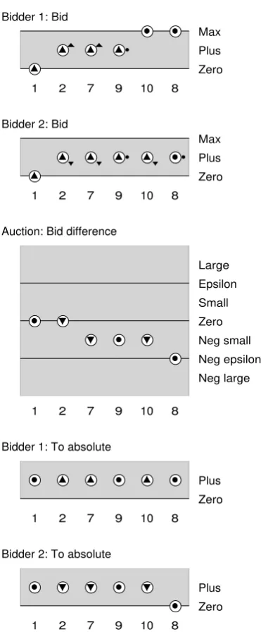
from zero by at least epsilon until the last state, namely state 8. Also until this last state, none of the bidders is the absolute winner. In the penultimate state, namely state 10, the first bidder reaches his maximum valuation, and, therefore, they stop increasing their bid. The second bidder then increases their offer until they become the absolute winner.

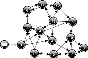
Figure 2.10: The state graph of the model for the two bidders continuous English Auction, together with the initial scenario from Figure 2.2.

From the state graph, notice that state 8 is the only state without any suc-cessors. This is, therefore, the only equilibrium point of the auction, that is the only point when bidders do not have an incentive to change their offer. Since, in this state, the revenue, i.e. highest offer, equals the second highest valuation plus

Epsilon, and Epsilon is arbitrarily small, the result of the simulation is in accor-dance with Vickrey’s theorem (Vickrey, 1961). This theorem also proves that the expected revenue for the English Auction equals the second highest valuation.

(31)

2.3. Reasoning Engine 23

Bidder 1: Bid

Zero Plus Max

1 2 7 9 10 8

Bidder 2: Bid

Zero Plus Max

1 2 7 9 10 8

Auction: Bid difference

Neg large Neg epsilon Neg small Zero Small Epsilon Large

1 2 7 9 10 8

Bidder 1: To absolute

Zero Plus

1 2 7 9 10 8

Bidder 2: To absolute

Zero Plus

[image:31.595.204.390.109.558.2]

1 2 7 9 10 8

Figure 2.11: A path in the state graph from Figure 2.10.

2.3 Reasoning Engine

(32)

2.3.1 Outline

As explained in Section 2.1, a simulation is based on a given library of model fragments, which encode the general behaviour of the system, and on a scenario, which provides some information about a state the system could be in. Given these two elements, the engine firstly extends the provided scenario to one or more initial states, depending on whether the scenario was ambiguous. After this, for each state, its successors are found and added to the state-graph, together with the respective transitions.

[image:32.595.97.502.395.479.2]

The process of finding states and transitions is done in phases. Firstly, when a state is created, either as an extension of a scenario or as a successor of an existing state, its state is marked asinterpreted. Next, the simple terminations of the state are identified and the state is marked as terminated. Then, the eligible compound terminations are found, via a procedure that we will later describe, and the state is marked asordered. Lastly, the state becomesclosed when its valid successors obtained from the short-listed compound terminations are identified, and the respective transitions are found. At this point, it is known that the state at hand cannot be further continued to a successor. Figure 2.12 gives an visualisation of these phases of a state.

Figure 2.12: The phases of a state in the state-graph generation process

Each of the three phases has its own procedure. Firstly, in order to identify the simple terminations, and hence change the phase of the current state from interpreted to terminated, the rules shown in Table 2.2 are used. Secondly, the state becomes ordered by finding combinations of simple terminations that might lead to valid successors. More precisely, a series of rules that will be later intro-duced is used to early identify incompatible combinations of simple terminations, and hence reduce the number of eligible compound terminations. Lastly, the state becomes closed. This is the most complex phase in terms of the number of steps involved, as it contains continuity checks, the identification of the new applicable model fragments, and, in case the current compound termination results in a successor, a check to see if that state already exists in the graph. From the per-spective of our axiomatisation, for each compound termination T, in this phase, the engine first finds the transition scenario from s with T. Then it applies the continuity criterion, and stabilises the state.

(33)

the context of this thesis. One is model fragment selection, which does repeated checks for finding active model fragments (Bredeweg et al., 2009). The other one is inequality reasoning, which verifies the consistency of a scenario with a given model fragment function. The latter one will be further discussed at the end of this section.

From the three phases, a closer examination is only needed for the ordering one. The termination phase is already clarified due to the axiomatisation from Section 2.1. Regarding the closing phase, for the purpose of this thesis there are only two important aspects to mention. First, it requires at least two calls to the inequality reasoner for each eligible compound termination. Second, given a transition scenario and a compound termination, it gives a continuous and stable extension of the scenario with the termination, i.e. it finds valid successors.

Having provided a general overview of the reasoning engine, the remaining two subsections focus on further discussing some of the procedures involved, namely inequality reasoning and state ordering.

2.3.2 Inequality Reasoner

A key component of the engine is the inequality reasoner. This is a procedure that given a set of relations, S, together with an extra relation r, tries to add the relationrto the setS. There are three possible answer based on the compatibility between r and S. First, if S and r form an inconsistent system, then r cannot be added to the system. Second, ifr can be inferred fromS, then it is deducible, so there is no need to add it to the system. Third, if r is consistent with S but not inferable, then it is added to S. For the purpose of this thesis, the inequality reasoner will be only used to check for consistencies of relation sets. Obviously, this can be done. To check if a set S is consistent, S together with a tautology, such as 0 = 0 is passed to the inequality reasoner. Then S is consistent if and only if 0 = 0 is found to be deducible.

Since, at an internal level, the information in models and scenarios can be represented by qualitative systems of (in)equalities, the inequality reasoning pro-cedure is essential. It is always used at least twice in the closing of a state for each eligible compound termination. In addition, it is occasionally also used in the ordering phase, as will be discussed in the next subsection.

Even though extremely useful, inequality reasoning is computationally expen-sive. This is because the detection of all implicit contradictions requires the full transitive closure of the internal system of (in)equalities, together with addition and subtraction inferences (Bredeweg et al., 2009). In fact, according to Veber et al. (2004), the problem of finding a solution for system of (in)equalities isNP -complete, as SAT, the satisfiability problem for sets of clauses, reduces to this inequality reasoning problem.

(34)

state uses inequality reasoning, this is in turn also time expensive. Therefore, reducing the number of transition scenarios requiring closing is useful. Hence, lowering the number of eligible compound terminations found in the ordering phase corresponds to lowering the time required by the simulation.

In the next subsection, some methods for reducing eligible combinations cur-rently in use are presented.

2.3.3 Ordering a State

Within this subsection, it is assumed that there is a terminated state, that is a state together with a set of its simple terminations, which will be denoted by (s = hE,val, <,≤,=i,T). Since the total number of compound termination is exponential in the number of simple terminations, O 2|T |, the engine cannot analyse all the possible combinations. Hence, some rules must be used in order to lower this amount. The aim of this phase is to find a short-list of eligible com-pound terminations. In the current subsection, the approach of Garp3 (Bredeweg et al., 2009) is presented.

To form this short-list, the epsilon ordering rule is firstly used. As explained in the previous section, the set of terminations T is partitioned in the class of immediate and non-immediate terminations. If the first one is non-empty, then all the compound terminations must be a subset of it, while if it is empty, the compound terminations are formed from non-immediate simple ones.

Secondly, three more rules are used in order to infer constants on the termi-nation combitermi-nations. In general, these rules will be referred to as combination concepts. A combination concept function, for a given state and model fragment function, is a function, comb, that, given a set of simple terminations, say S, returns a set ofcombination constraints, that is of logical relations that constrain the possible ways of combining the terminations in S. One example of such a rule is t1 ∈ T ↔ t2 ∈ T, which says that t1 and t2 must co-occur. This will

be abbreviated as t1 ↔ t2 Another example is when t1 and t2 are incompatible,

which is given by the relation t1 ∈/ T ∨t2 ∈/ T, and is abbreviated as ¬t1∨ ¬t2. One combination concept is the mutually exclusive terminations constraint. This rule identifies terminations that might not appear together, which may hap-pen in the case of terminations with assumed causes. For example, if a bid difference is at Epsilon with an unknown derivative, then there could be as-sumed terminations that either change it to Small orLarge, and these two can-not be combined. That is, combinations of terminations with causes such as (assumed to interval above, Q) and (assumed to interval below, Q), are not al-lowed.

(35)

is the pair ((P1, v1),(P2, v2)) for some parametersP1, P2, and values v1, v2 within

their magnitude spaces, vi ∈ MPi. As a reminder, this means that whenever P1

has value v1, P2 must have the corresponding value v2. Suppose moreover that

the value assertion of s, that is val, is such that val(P1) = v1, and val(P2) = v2.

Then, if there is no simple termination changing the value of P1, either above or below, then any simple termination changing the value ofP2, if such exists, must

not occur in eligible compound terminations. In other words, if T contains a termination changing the value of P2 but none changing the value of P1, then the first one cannot be used in any combination. This is because P1 cannot change

value, so it will remain at v1, and by the value correspondence, P2 should not

change either from v2.

Table 2.3 presents an overview of the rules used in the correspondence order-ing. As in the example before, those are under the assumption of an existing correspondence ((P1, v1),(P2, v2)). This table analyses the cases when the two

parameters are both at the corresponding values, both not at the corresponding values, and when onlyP2 is at the corresponding valuev2. The fourth case, when

onlyP1is at the corresponding value, that is whenval(P1) =v1 andval(P2)6=v2,

cannot appear, as it does not satisfy the correspondence constraint, so s is not stable, and hence it cannot be a state.

The last combination concept in use is the mathematical ordering. This is a rule that checks if combinations of changes can occur from the perspective of relation-correctness. More precisely, if we have two parameters,P1, P2, and three

terminations, a value ti termination for each Pi and an inequality termination t3

for the pair (P1, P2), then there are certain bounds on how these terminations

can appear together. For instance, if currently P1 = P2, then a change of

in-equality can only appear together with at least a change in the values of the two parameters, i.e. t3 →t1 ∨t2.

To apply this, the engine takes every pair of quantities that have a specified relation between them and that is still valid under the previous two combination concepts. Since this step is computationally demanding, it is actually important to be the last one that is checked, in order to have the least amount of valid com-binations as input. In addition, every considered pair needs to have inequality constraints on the landmarks that could be reached through combinations. Fi-nally, the inequality reasoner is used to check which combinations of terminations are valid.

Lastly, after using all these three combination concepts, the constraint cross product of the simple terminations is taken. This means that the engine finds the subset of the cross product such that all the compound terminations in this subset satisfy the conditions returned by the combination concept function, that is the conditions withincomb(T).

(36)

Value assertion

Combination constraint

Description

val(P1) =v1,

val(P2) =v2

t2 →t1 If P1 and P2 are both at the corresponding

values, then P2 cannot change value alone. In the particular case when there are no ter-minations changing the value of P1, then P2

cannot change at all, so any value termina-tion onP2 can be eliminated.

val(P1) =v10,

val(P2) =v20

t1 →t2 If P1 and P2 are both at adjacent values to

the corresponding ones, thenP1 cannot move

alone to the corresponding value. Similarly, when there are no terminations changing the value of P2, then P1 cannot change at all,

so any value termination onP1 can be

elim-inated.

val(P1) =v₁0,

val(P2) =v2

¬t1∨ ¬t2 IfP2is at the corresponding value, whileP1is at an adjacent one,P1 cannot change to the

corresponding value, while P2 moves away

from it.

Table 2.3: Correspondence ordering constrains for parameters P1, P2, where v1 ∈ MP1 corresponds to v2 ∈ MP2. Each v

0

i is a value within MPi that is adjacent

to vi (either smaller or larger), and each ti is a termination on Pi with value or

derivative causes that change the parameters either from vi to vi0, or the other

way around.

constraint cross product is further reduced by eliminating all the compound ter-minations that are a subset of another compound termination.

This finalises the explanation of how the eligible compound terminations are selected in Garp3. The next section analyses the impact of using these combina-tion concepts by considering a large simulacombina-tion example.

2.4 A Large Simulation

(37)

2.4. A Large Simulation 29

in the simulation of this model. The most attention is paid to state 3, as this is also used as an example at the end of Chapter 5.

Quantity Magnitude Derivative

ConcentrationActivenzyme Plus +

ConcentrationFreeenzyme Plus +

ConcentrationProduct Plus +

ConcentrationSubstrat Max 0

ConcentrationSurfaceenzyme Plus +

Quant enzyme_Enzyme Total 0

Quantity of submol_Sugar Total 0

Rate inAdditionenzyme Plus −

RateadsSurfaceenzyme Plus +

RatecatActivenzyme Plus +

Ratecomp_Activenzyme Plus +

RatedesFreeenzyme Plus +

Rateoff_Activenzyme Plus +

Surface available_Substrat Plus −

Surface covered_Substrat Plus +

[image:37.595.168.434.162.490.2]

Surface max_Substrat Max 0

Table 2.4: Cellulose Hydrolysis: values of quantities in state 3.

As an initial scenario, the basic enzymatic reaction restart is considered. The resulting state graph has 83 states, and takes almost two days to be fully com-puted. 1 _{For the first 14 states of this simulation, we used the profiler procedure}

in SWIProlog (Graham et al., 2004) to record the CPU times for each phase in simulating in the state. As expected from the theoretical complexity results, for all these states the most time was spent in the closing of a state; while the terminating and ordering phases were always carried out in less than 1 minute, some closing of states took almost 1 hour. For instance, one state with only two valid successors but 255 compound terminations took 34 minutes to close. In ad-dition, also in accordance with the theoretical results, most time was spent in the inequality reasoner (more than 80%). This suggests that, for practical reasons as

1_{These results were obtained on an Intel Core i5 1.7GHz processor, with 4 GB of RAM}

(38)

Label Simple termination cause

1 (to point below,Surface available_Substrat) 2 (to point above,ConcentrationSurfaceenzyme)

3 (to point above,Surface covered_Substrat) 4 (to point above,ConcentrationProduct)

5 (to point above,ConcentrationFreeenzyme)

6 (to point below,Rate inAdditionenzyme)

7 (to point above,ConcentrationActivenzyme)

8 (assumed derivative up to stable,ConcentrationSurfaceenzyme)

9 (assumed derivative up to stable,ConcentrationFreeenzyme)

10 (assumed derivative up to stable,ConcentrationActivenzyme)

11 (assumed derivative up to stable,RateadsSurfaceenzyme)

Table 2.5: Cellulose Hydrolysis: simple terminations for state 3.

well, it would be useful to lower the number of calls to the inequality reasoner. Let us now consider a particular state, which has valuation in accordance with Table 2.4. From this, 11 simple terminations are found (see Table 2.5). One can check that these are in accordance with the termination validity criteria from Table 2.2. The number of eligible compound terminations identified is 511. Notice that this is reduced as, by combining all the simple terminations, 211₋_{1 =}

2047 compound terminations would have been found. Figure 2.13 shows the development of the state graph throughout these phases.

(a) The extension of the initial scenario.

(b) The simple termina-tions.

(c) The successors.

(39)

2.5. Conclusion 31

2.5 Conclusion

To summarise, this chapter made four contributions. First, and most importantly, it has introduced a new axiomatisation that focuses more on the simulation as-pects than the previous formalisation attempts (Bredeweg et al., 2009; Liem, 2013; Weld, 1988). It used clear notations and definitions for simple terminations, which are possible next-state developments of a system, and compound terminations, which correspond to simultaneous developments. This leads to clear definitions for the simulation output, i.e. state graph, which is the overview of the possible future behaviours of the system. All those definitions are indispensable in order to perform a theoretical analysis of the process-oriented qualitative simulations, in their current form. Second, since this is done in the context of the earlier formalisations, this chapter also serves as a literature review.

Third, for clarifying those definitions, the continuous English Auction with two bidders model was used. This is a novel example extending the applications of qualitative simulations to the field of Auction Theory. The results of the sim-ulation were in accordance with the theoretical ones in the field, hence implying the correctness of our model.

Fourth, Garp3 (Bredeweg et al., 2009) was used as example of a qualitative reasoning engine. Its inner workings were illustrated by means of a large example of cellulose hydrolysis (Kansou et al., 2017). Three important phases were iden-tified for obtaining successors, namely termination, ordering, and closing. Also, a very important procedure within simulation is the inequality reasoner, which checks the consistency of systems of qualitative (in)equalities. This was shown by Veber et al. (2004) to beNP-complete. The brief practical case analysis car-ried out in the last section revealed that this theoretical result correlates with slow running times. As a result, since the closing phase requires multiple calls to the inequality reasoner, the number of compound terminations requiring anal-ysis during closing should be lowered. This can be done by better using sparse knowledge for early identification of incompatible compound terminations.

(40)

(41)

Chapter 3 Criteria for Simulation Consistency

As already mentioned in the previous chapter, data is sparse in qualitative models, in the sense that not all valid relations in the model are made explicit. Conse-quently, the simulation is based on incomplete information, leading in some cases to incoherent results. The goal of this chapter is to use the axiomatisation created before in order to identify incoherences, as well as to find solutions for eliminating them.

Three principles of coherence are discussed. The first section investigates model consistency, that is whether transitions in simulation results are in accor-dance with the constraints of the system. The second section considers paths in the resulting state graph. As a principle, each state graph should be path consistent, meaning that the information recorded in successions of states should describe a coherent behaviour. The last section discusses consistency from the perspective of inexplicit (in)equalities, as, even when relations are not explicit but only inferable from either a scenario or a model fragment, the state graph should still be consistent with them.

3.1 Model Consistency

(42)

3.1.1 Dependency Consistency

As already mentioned, dependency consistency is the principle which states that each transition should be in accordance with the dependency relations given by the model fragment function, that is with the influences and proportionalities. Because each state is stable, it is clear that the influence and proportionality balances are respected. However, dependencies could provide other information as well.

To see this, first consider an example. Suppose there is a meeting room in which people enter via an entrance corridor, and from which they exit via an exit corridor. In terms of qualitative modelling, this means that we have the entity room with three quantities: the number of people in the room, to which we will refer to asNo room, the number of people in the entrance corridor,No entrance, and the number of people in the exit one,No exit. In addition, there is a positive influence from No entrance to No room, as if there are people at the entrance, then they will go in the room, so the number of people in the room will increase (if none of them are exiting). Similarly, there is a negative influence fromNo exit

toNo room.

The model fragment for the system described above is shown in Figure 3.1. The conditionals, which, in this case, are the entityRoomtogether with its three quantities, are drawn in red. The causal ingredients returned by the model frag-ment, namely the two inferences, are pictured in blue.

Figure 3.1: The model fragment for a room with entrance and exit corridors.

(43)

3.1. Model Consistency 35

Figure 3.2: An initial scenario for the meeting room model.

Next, the evolution of this situation is analysed. To begin with, accord-ing to the scenario, the tendency of the number of people in the room is com-pletely balanced at 0 by the ones entering and the ones exiting. So, dNo room =

f(No entrance)−g(No exit). Since dNo room = 0, then we should have f(No entrance) =g(No exit). Moreover, as the derivative ofNo exitis positive andgis strictly monotonous, g(No exit) is increasing, so we will immediately have in the next state f(No entrance)< g(No exit), and, hence, dNo room <0. Therefore, we would expect an unique successor of the state extending the given scenario, which would be the same as the current state, but withdNo room =−. However, without considering the second order derivatives, this is not the case, because for each of the three values ofdNo room, the resulting state is stable and continuous, but neither is justified by an simple termination according to Table 2.2. This can also be exemplified by running this simulation in Garp3 with the default training preferences. According to this, no successors of state 1, the state extending the initial scenario from Figure 3.2, can be found.

This is a general issue extending beyond our example. Such a problem might appear whenever there is a quantity with at least two incoming dependencies. One way of fixing it is to consider second order derivatives. To understand why doing so solves the issue, we return to the example before. Now, when extending the given scenario, the second order derivatives of the three quantities will also be identified. Hence, ddNo room = df(No entrance)−dg(No exit) is deduced sincedNo room =f(No entrance)−g(No exit). Becausef andg are continuous and strictly monotonous, ddNo room = 0−minus =minus. As now the deriva-tive of dNo room is negative, this will trigger only one derivative termination on

(44)

simulation preferences.

Another way of producing the expected behaviour would be to add extra causes for terminations based on the model fragment function. More precisely, for a state s = hE,val, <,≤,=i, the Table 2.1 is extended with the four causes in Table 3.1. As before, the starred causes are for immediate terminations. The associated sets of constraints and results set are presented in Table 3.2.

Class of causes Type of cause

Model consistency causes (mc derivative stable to down, P)* (mc derivative stable to up, P)∗ (mc derivative down to stable, P) (mc derivative up to stable, P)

Table 3.1: Model consistency causes

For clarity purposes, let us now explain the second validity criteria in Table 3.2. Because of the inference and proportionality balance, we have that

dP = X

Pi∈P r+

fi(dPi)−

X

Pj∈P r−

fj(dPj) +

X

Pk∈In+

fk(Pk)−

X

Pu∈In−

fu(Pu),

where P r+ ={Pi|(Pi, P)∈P+}, P r− ={Pj|(Pj, P)∈P−},In+ ={Pk|(Pk, P)∈

I+}, and In− ={Pu|(Pu, P)∈ I−}. So if all dPi, Pk are steady or increasing, all

dPj, Pu are steady or decreasing, and at least one of them all have the tendency

to change, then P should immediately have the tendency to increase. That is, there is a termination with dP = +.

In the meeting room example, there are two influences to No room. The positive one comes from a steady quantity, while the negative one comes from an increasing quantity. This state description matches the constraints of (mc derivative stable to down,No room), which is an immediate termination chang-ing the value of dNo room to −.

(45)

3.1. Model Consistency 37

Cause type Elements of cond(t) Elements of results set

(mc derivative stable to down, P)

val(dP) = 0

∀(P0, P)∈P+ val(ddP0)≤0 defined ∀(P0, P)∈P− val(ddP0)≥0 defined

∀(P0, P)∈I+ val(dP0)≤0 defined

∀(P0, P)∈I− val(dP0)≥0 defined

at least one of the inequalities is strict

val(dP) = −

(mc derivative stable to up, P)

val(dP) = 0

∀(P0, P)∈P+ val(ddP0)≥0 defined

∀(P0, P)∈P− val(ddP0)≤0 defined

∀(P0, P)∈I+ val(dP0)≥0 defined

∀(P0, P)∈I− val(dP0)≤0 defined

val(dP) = +

(mc derivative down to stable, P)

val(dP) = −

∀(P0, P)∈P+ val(ddP0)≥0 defined ∀(P0, P)∈P− val(ddP0)≤0 defined

∀(P0, P)∈I+ val(dP0)≥0 defined

∀(P0, P)∈I− val(dP0)≤0 defined

val(dP) = 0

(mc derivative up to stable, P)

val(dP) = +

∀(P0, P)∈P+ val(ddP0)≤0 defined

∀(P0, P)∈P− val(ddP0)≥0 defined

∀(P0, P)∈I+ val(dP0)≤0 defined

∀(P0, P)∈I− val(dP0)≥0 defined

[image:45.595.97.498.115.527.2]

val(dP) = 0

Table 3.2: Termination validity criteria for model consistency causes for state s

with active causal ingredients P+, P−, I+, I−.

3.1.2 Relation Consistency

Besides dependencies, other model fragment ingredients that should be respected are the relations between parameters. The ones that are made explicit in the system are trivially considered, as it is a requirement for the stability of states. However, the relations that are inferable from the explicit ones by taking deriva-tives are not necessarily considered. In general, if there is an equality between terms, then the relation obtained by taking derivatives should hold as well.