Extracting partition statistics from semistructured data

Extracting Partition Statistics from

Semistructured Data

John N. Wilson

Richard Gourlay

Robert Japp

Mathias Neum¨uller

Department of Computer and Information Sciences

University of Strathclyde, Glasgow, UK

{

jnw,rsg,rpj,mathias

}

@cis.strath.ac.uk

Abstract

The effective grouping, orpartitioning, of semistructured

data is of fundamental importance when providing support for queries. Partitions allow items within the data set that share common structural properties to be identified effi-ciently. This allows queries that make use of these prop-erties, such as branching path expressions, to be acceler-ated. Here, we evaluate the effectiveness of several parti-tioning techniques by establishing the number of partitions that each scheme can identify over a given data set. In par-ticular, we explore the use of parameterised indexes, based upon the notion of forward and backward bisimilarity, as a means of partitioning semistructured data; demonstrating that even restricted instances of such indexes can be used to identify the majority of relevant partitions in the data.

1

Introduction

Efficient resolution ofbranching path expressionsover

XML data requires that data items having a structure that matches thatspecified by the query can be identified with-out traversing the complete data set. This can be achieved with a suitable form of index graph. Such graphs can pro-vide a structural summary of the complete data set and allow data items with similar structure (and semantics) to be col-lected together and accessed efficiently. Consequently, in-dex graphs implicitly define a partitioning of the data, with the number, and nature, of partitions identified varying with choice of indexing technique. In this paper, we explore the effectiveness of a number of forms of index graph through an exploration of the number of partitions that each index can identify over a given data set.

The different forms of index that can be used with

semi-structured data each define a set ofpartitionsover the data.

Each vertex on the index graph corresponds to exactly one

partition, with all data therein sharing some notion of com-mon structural properties. The size of the index graph, and therefore the number of partitions identified, varies dramat-ically with choice of indexing technique. There is a trade-off between the size of the index graph and accuracy con-sequently the choice of index and the number of partitions identified, will vary considerably depending on which form of index has been selected.

Constructing a suitable index graph, and identifying a set of partitions, is a fundamental step in the efficient process-ing of semistructured data. In addition to the benefits of efficient access provided by the index graph, partitions pro-vide a valuable opportunity for optimisation. Firstly, it is likely that data within a given partition will be accessed to-gether. Secondly, partitions capture regular aspects of the data set, presenting an opportunity to exploit techniques aimed at such data (which have been extensively studied for the relational model). Index graphs, and the partitions that they identify, are central to the efficient processing of XML and can be used as the basis of query processing models in the absence of globally valid schemata or when cost-based optimisers are unavailable.

The remainder of this paper is structured as follows. Sec-tion 2 summarises the necessary concepts and terminology, while Section 3 describes a number of techniques for par-titioning semistructured data. Section 4 presents the main contribution of this paper: an evaluation of how effective different indexing techniques are at identifying partitions of the data. Section 5 concludes the paper.

2

Background

The data graph representation of semistructured data is

adirected node-labelled graph. The vertices of this graph

it is only when additional relationships, such as those en-coded using ID:IDREF references, are included that a graph containing cycles can be obtained. Here, we refer to a tree view of the data that is both a spanning tree and is rooted at

the root vertex as adistinguished spanning tree. The forms

of index graph of interest here are all targeted at path ex-pressions (i.e. they do not index the values of the atomic data) and provide a graph derived from the data graph that can associate multiple data items with a single vertex.

Branching path expressionsare a form of query that can

be performed over a data graph. These queries are

com-prised of a sequence of labels (alabel path), and can

con-tain both forward and backward separators. Evaluating such a query consists of finding all vertices on the data graph that have a path leading to them matching the path given by the labels with forward separators (this is referred to as the

primary path) that also satisfy the conditions given by the

backward separators. If a given index graph is smaller than the data graph it summarises, then it is possible to evaluate a query more efficiently using the index than it would be to traverse the complete data set.

The use ofbisimilarityas a means of partitioning

semi-structured data was first demonstrated by Buneman et al. [1]. Such indexes group vertices on the data graph ac-cording to the equality of the complete set of outgoing and incoming edges to a given vertex. This produces a refined set of partitions over a given data set that can be used as an aid to the efficient processing of branching path expres-sions. However, such index graphs can become too large to be useful. Kaushik et al. [5] introduce a parameterised index based upon bisimilarity, with a view to using such pa-rameters to limit the size of the index graph. More recently, He and Yang [4] proposed a multi-resolution index upon bisimilarity: a form of index with the degree of bisimilarity varied according to the needs of each node.

3

Partitioning Techniques

Partitions can be categorised in one of three ways (de-pending on the type of vertices contained therein). Firstly, a partition comprised solely of vertices representing atomic

data is said to be an atomic partition. Secondly, a

parti-tion that contains only complex vertices, those vertices that combine the information stored in other vertices by means

of a set of outgoing edges, is said to be acomplex partition.

Finally, a partition that contains both atomic and complex

vertices is said to be amixed partition. Such distinctions

will be considered when contrasting different partitioning schemes.

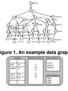
Technique 1 (Label Partitions)This is the simplest par-titioning technique discussed here. For a given data set (Fig-ure 1), all vertices carrying an identical label are grouped together. Using this approach, there will be exactly one

name name class

cis ROOT

teaching

class prerequisite

assistant

staff people

researcher

student staff

research

name lecturer

project

lecturer

&0

&16 &1

&2 &3 &4

&5 &6 &13 &11

&12 &14

&15 phone

name name

phone phone

&7

&17 &18

&19 &20 &8

name

&24 &9

&21 &22

&10

&23

"Databases"

"S.A.D." "3839" "Mathias"

"3590" "John"

"3584" "Domains" "Sotirios"

&25 &26

&27 &28

&29 &30

&31 &32

&33

Figure 1. An example data graph

… T7 T8 C1 / T9 C2 / …

… S.A.D. Sotirios Mathias …

3839 3590 3584 Data Container 1

Data Container 2 Structure Container

… …

phone T9 staff T6 studentT7 name T8

… … Tag Map

Figure 2. XMill containers.

atomic partition and one complex partition for each source-specific tag present in the data graph (including the root ver-tex).

Technique 2 (Parent Partitions) This technique is based on the equality of the label of a node’s parent node in the distinct spanning tree system [7]. A vertex on a data graph may have more than one incoming edge (par-ent node), so it becomes possible for a node to be pres(par-ent in more than one partition. The total number of partitions that can be identified is bounded by the size of the label alpha-bet. Since the root vertex has no incoming edge it does not belong to any partition. Inversely, there is no partition

cor-responding to the tag labelDATA, as atomic vertices have

no outgoing edges.

Figure 2 illustrates the transformation of our example data graph as used with XMill. This approach causes all data items representing a ‘name’ to be merged into one atomic partition, regardless of whether they are the names of people, projects or courses. This effect of combining

un-related information is referred to aspartition mixing.

Technique 3 (Path Partitions) This partitioning tech-nique attempts to avoid partition mixing by partitioning the vertex set based upon the entire path from the root node to a given vertex. This may result in a given vertex being part of more than one partition. In fact, cyclic graphs will result in an unbounded number of partitions being identified. How-ever, the equivalent technique based upon the distinguished spanning tree is bounded by the size of the node set giv-ing a usable definition of partitiongiv-ing. This is equivalent to

the strong DataGuide [3] and can result inpartition splitting

(Figure 3).

c1cis

c0ROOT

c3people

c2teaching

c5class c6staff c7student c8project c9name

c4research

c13name c15name c17name c10lecturer c12assistant c14phone c16phone c18researcher

a19DATA a20DATA a24DATA

a23DATA

a21DATA a22DATA

prerequisite c11

Figure 3. Strong

DataGuide.

c0

c1

c2

c3

c4

a5

&1 cis &0 ROOT

&3 people &2 teaching

&5 class &6 class &7 staff &8 student&9 staff &10 project

&11 name

&4 research

&14name

&19 name

&21 name &23 name &12 lecturer

&18 phone &20 phone &22 phone &13 prerequisite &24 researcher

&25 “Databases”&26 “S.A.D.”

&27 “Sotirios” &29 “Mathias” &28“3839”

&33 “Domains” &32 “3584” &30“3590”

&31 “John” name

&17 assistant &16

lecturer &15

Figure 4. Depth parti-tions.

class

cis ROOT

teaching

class prerequisite

name lecturer assistant staff name

DATA people

researcher student staff

phone phone DATA name

project research

name c

c

c

c c c

c c

c

c c c c c

c c c c c

22

c c

0

1

2 3 4

14 20

5 6 7 8 9 10

11 12

13

15 17 18 16 19

a a₂₄

Figure 5. The A(1)-index graph.

name name c₁₂lecturer

class

cis ROOT

teaching

class prerequisite

assistant staff name

DATA people

researcher student staff

phone phone DATA name

research

name c

c

c

c c c

c c

c

c c c c c

c c c c c

0

1

2 3 4

14 20

5 6 7 8 9 10

13

17 18 19 20 21

23 24

a c₁₄

c₁₅lecturer

11

c

project

a a

Figure 6. The (1,1)-F+B-Index graph.

together. Although such a partitioning may initially seem to be of limited use, certain queries can be accelerated with an index based upon such a partitioning. For example, the

query/*/*/*, can be resolved efficiently using this

tech-nique. If this technique is used on the graph view of the data then, as was the case with Path Partitions, an unbounded number of partitions can be identified. Given that the parti-tions identified do not take account of node labelling, mixed partitions can be identified. Figure 4 shows such a partition-ing imposed on the data graph.

Technique 5 (Skeleton Partitions) This technique is based on the concept of forward bisimilarity of a node [2], i.e. the equality of the collection of outgoing paths. This technique states that two nodes in the tree are said to be bisimilar if they have the same label and the same ordered sequence of bisimilar child nodes. This allows common substructures in a document to be identified, for example,

the two staff nodes shown in Figure 1; however, this

technique splits the twoclassnodes because of the

dif-ferences in their respective sub-trees. Given that only out-going edges are considered when computing bisimilarity, all atomic data is grouped in a single atomic partition.

Technique 6 (Local Backward Bisimilarity Parti-tions)Here the entire set of incoming edges is used to de-termine the partition of each node [6]. This gives an index that is similar to that of path partitioning, whilst avoiding nodes being present in multiple partitions based on each in-coming edge. Since, in practice, path expressions are often of limited length, the lengths of the paths used when

calcu-c1cis c0ROOT

c3people c2teaching

c5class c6class c7staff c8student c9project c4research

c13name c14phone c11lecturer

c12assistant

c10prerequisite

c15researcher

a16DATA

Figure 7. The skeleton representation.

Xmark PubMed

MAGE Ensembl Rat

Source Size (MB) 10 31 36 75

www.ncbi.nlm.nih.gov/entrez www.ensembl.org www.mged.org Synthetic data, scale factor 0.1 Note

Figure 8. Data structures investigated.

lating the bisimilarity can also be limited. The definition of bisimilarity then becomes recursive, stating that a vertex is

k-bisimilar to another if they have equal labels and have the

same set of incoming edges from vertices that are(k−1)

-bisimilar. Thus, the parameterkcan be used to control the

balance between index size and index coverage. Figure 5 shows the index graph of the example source based on 1-bisimilarity. Again, every vertex defines a partition of the

data set. The twostaffvertices that were contained in a

single partition when using skeleton partitions are now split As seen previously, all names are merged into a single par-tition regardless of whether they refer to people, projects

or courses. Increasing the value ofkwould overcome this

limitation.

Technique 7 (Forward and Backward Bisimilarity Partitions)This method combines the structural properties identified by techniques such as skeleton partitions, with the contextual properties that can be identified using back-ward bisimilarity [5]. The resulting index graph is covering for general branching path expressions without value pred-icates. As with local backward bisimilarity, the lengths of

paths considered can be limited. Here, two parameters,kb

andkf, that restrict the lengths of incoming and outgoing

paths respectively, can be used to reduce the complexity of the final index graph. Figure 6 shows the index graph based

on (1,1)-F+B-bisimilarity, Thenameandlecturer

ver-tices occurring belowclassvertices have been split,

al-though their incoming paths of length one are identical. This is because they can be distinguished based on their siblings by using a branching path expression whose length does not exceed one. For example, the branching path

ex-pression class[/prerequisite]/name selects vertex

&11but not vertex&14, which were combined in partition

c11in Figure 5 but are split into the partitionsc11andc14.

4

Partition Statistics

Xmark PubMed

MAGE 3,139,711 2,556,204 1,288,555 322,327 Ensembl Rat

Xmark PubMed

MAGE 3,139,711 2,556,204 1,288,555 322,327 Ensembl Rat

Xmark PubMed

MAGE 3,139,711 2,556,204 1,288,555 322,327 Ensembl Rat

Xmark PubMed

MAGE 3,139,711 2,556,204 1,288,555 322,327 Ensembl Rat

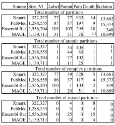
Total number of partitions Source Size |V| Label Parent Path Depth Skeleton

77 87 103

31 31 103 87

77 13,662 15,374 340 10,699 14

9 933 197 295

76 11 18

1 1 1 1

1 1 1 1

1 1 1 1 405

80 102 25 34 44 77 11 77 86 103 31

39 37 1 20

528 117 103 51

5 4 2 6

15,373 13,661 339 10,689 0

0 0 0

0 0 00

0 0 0 0 4 5 25 0

8 4 15 4 Total number of atomic partitions

Total number of complex partitions

Total number of mixed partitions

Figure 9. Static partitions counts.

technique and the complexity of the underlying data source.

Partition Techniques 1–5 are classified asfixed-partitioning

techniques, in that they do not support the use of

param-eters to influence the operation of the algorithm. With

parameterised-partitioningtechniques however, a range of

parameter combinations are possible.

4.1

Fixed-Partitioning Statistics

Figure 9 shows the number of distinct partitions that can be identified over our sample data when using partition-ing Techniques 1–5 (the partitionpartition-ing techniques that do not make use of parameters). The results shown in Figure 9 clearly demonstrate that competing partitioning techniques produce significantly different numbers of partitions for a given data.

In contrast to the regular structure of the Ensembl file (Figure 9), the XMark data exhibits few indications of a reg-ular structure since its data, by design, is convoluted. This is indicated by the results presented in Figure 9. In the XMark data set there is no correspondence between the number of complex partitions identified by label partitioning and path partitioning (or indeed, any of the chosen schemes). A large number of partitions are identified using the skeleton parti-tioning technique, even though the size of the data graph is significantly smaller than the data graph of the other sam-ple documents. This is a consequence of similar elements occurring in many contexts in XMark generated files.

Of the remaining two example files, PubMed and MAGE, the results shown indicate that they do have some degree of varying content (i.e. tags appearing in differ-ent contexts), but that these real data sources do not have the same complexity as the synthetically generated XMark data. When using the skeleton partitioning technique, the number of partitions identified for the PubMed and MAGE files is comparable to that of the XMark data, although, again, it should be noted that there is a significant differ-ence in the size of the data sets.

With the exception of the regularly structured Ensembl file, the number of partitions identifiable using the

Skele-fw=0fw=1 fw=2fw=3 fw=4 fw=5 bw=0

bw=2 bw=4

0 50000 100000 150000 200000 250000 300000

Figure 10. XMark:

Depth= 1

fw=0 fw=1fw=2 fw=3 fw=4 fw=5 bw=0

bw=2 bw=4

0 50000 100000 150000 200000 250000 300000

Figure 11. XMark:

Depth= 3

ton technique greatly exceeds that of the more simple par-tition techniques. This suggests that techniques based upon bisimulation are likely to be the most applicable when ac-celerating branching path expressions or when clustering the data according to its context.

4.2

Parameterised-Partitioning Statistics

In contrast to partitioning Techniques 1–5, Techniques 6 and 7 define a family of partition structures, with one or more parameters being used to specify the exact nature of any given instance of the partitioning. Points in the param-eter space that correspond to either stable or rapidly chang-ing numbers of partitions are of interest. Knowledge of such points may be beneficial when automating parameter choice for such indexes. The sets of partitions that can be identified using Technique 6 (local backward bisimilarity) are a sub-set of the sub-sets of partitions that can be identified using Tech-nique 7 (forward and backward bisimilarity). Thus, only the results obtained using Technique 7 are given here.

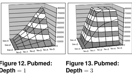
Figures 10 and 11 show the numbers of partitions ob-tained using a parameterised index for tree depths of 1 and 3. The results are shown as 3D-surfaces to allow the inter-action of the two parameters that control the size of the for-ward and backfor-ward bisimilarity to be seen. For any given

parameter combination (i, j), the set of partitions

identifi-able will include all partitions, or a refinement thereof, that

are identifiable using a lower value of i and/or j. Thus,

fw=0 fw=1fw=2 fw=3 fw=4 fw=5 bw=0

bw=2 bw=4

0 10000 20000 30000 40000 50000 60000 70000 80000

Figure 12. Pubmed:

Depth= 1

fw=0 fw=1fw=2 fw=3 fw=4 fw=5 bw=0

bw=2 bw=4

0 10000 20000 30000 40000 50000 60000 70000 80000

Figure 13. Pubmed:

Depth= 3

maximal number of partitions that could be identified us-ing this technique was very close to the number of vertices on the data graph: 285,372 partitions compared to 322,327 vertices on the data graph.

Figures 12 and 13 show the number of parameters that can be identified in the PubMed file using parameterised in-dexes of tree depths 1 and 3. In each case, the overall shape of the surfaces is similar to that obtained when using XMark data, although the surfaces are smoother and more closely resemble that which would be obtained over normally dis-tributed data. These smoother surfaces indicate that the structure of the PubMed data is more regular than that of XMark. The most significant difference in the data gath-ered over PubMed is that the maximal number of partitions identified is significantly smaller than the size of the origi-nal data graph: 73,874 partitions compared to a data graph of 1,288,555 vertices. Here, the full F&B index would be an order of magnitude smaller than the original data graph. Again, it can be seen that increasing the tree depth increases the rate at which the number of partitions grows.

Overall, it can be seen that even restricted instances of parameterised covering indexes have a complexity similar to that of the full F&B index [5]. Thus, if it is intended to provide a partitioning (index graph) that is smaller than that obtained with F&B index then the parameters for the pa-rameterised index can only be drawn from a limited range. When compared to the size of the data graph, the maxi-mal number of partitions identified over our two sample documents differed considerably. For XMark the maxi-mal number of partitions approaches the size of the data graph, whereas for PubMed the maximal number of parti-tions was an order of magnitude smaller than the size of the data graph. The input data determines whether it is viable to use higher values for the index parameters.

5

Conclusions

This paper summarised seven different techniques for partitioning semistructured data, contrasting their

effective-ness over various XML documents. As expected, the num-ber of identifiable partitions varied greatly with choice of partitioning technique; however, it was also found the num-ber of partitions varied greatly with the nature of the source data. Partitioning convoluted data sources, such as XMark data, can result in an index graph that approaches the com-plexity of the data graph. However, this was not found to be the case for real sources of semistructured data. Hence, in-dex graphs that potentially have a complexity equal to that of the data graph may well be viable over real data sources. Of the seven techniques described, those based upon bi-simulation (Techniques 5, 6 and 7) identified significantly more partitions for data with varying structure than the more simplistic partitioning techniques. Furthermore, employ-ing both forward and backward bisimulation (Technique 7) allowed significantly more partitions to be identified than is possible using bisimulation in only one direction (e.g. Skeleton Partitions). This suggests that partitioning on for-ward and backfor-ward bisimulation is the most appropriate technique for both accelerating branching path expressions and for clustering the atomic data according to context. Ad-ditionally, it was demonstrated that the number of partitions identified using parameterised indexes quickly approaches the maximum as the parameters controlling the forward and backward bisimilarity are increased. Hence, in situations were it is desired to limit the size of the index graph (and the number of partitions) then it will be necessary to draw values for these parameters from a restricted set of values.

References

[1] P. Buneman, S. Davidson, G. Hillebrand, and D. Suciu. A query language and optimisation techniques for unstructured data. InProc. of the 1996 ACM SIGMOD, pages 505–516, 1996.

[2] P. Buneman, M. Grohe, and C. Koch. Path queries on com-pressed XML. InProc. of 29th VLDB, pages 141–152, 2003. [3] R. Goldman and J. Widom. DataGuides: Enabling query for-mulation and optimization in semistructured databases. In

Proc. of 23rd VLDB, pages 436–445. Morgan Kaufmann, 1997.

[4] H. He and J. Yang. Multiresolution indexing of XML for fre-quent queries. InProc. of 20th ICDE, pages 683–694. IEEE Computer Society, 2004.

[5] R. Kaushik, P. Bohannon, J. Naughton, and H. Korth. Cover-ing indexes for branchCover-ing path queries. InProc. of the 2002 ACM SIGMOD, pages 133–144, 2002.

[6] R. Kaushik, P. Shenoy, P. Bohannon, and E. Gudes. Ex-ploiting local similarity for indexing paths in graph-structured data. InProc. of the 18th ICDE, pages 129–140, 2002. [7] H. Liefke and D. Suciu. XMill: An efficient compressor for