The ERA-EDTA cohort study—comparison of methods to predict survival on renal replacement therapy

(1)

doi:10.1093/ndt/gfi326

Advance Access publication 8 December 2005

Original Article

The ERA-EDTA cohort study—comparison of methods

to predict survival on renal replacement therapy

Colin C. Geddes

1

, Paul C. W. van Dijk

5

, Stephen McArthur

3

, Wendy Metcalfe

4

, Kitty J. Jager

5

,

Aeilko H. Zwinderman

6

, Michael Mooney

3

, Jonathan G. Fox

2

and Keith Simpson

2

1

Renal Unit, Western Inﬁrmary,2Renal Unit, Glasgow Royal Inﬁrmary, 3Engineering Department,

University of Strathclyde, Glasgow,4Renal Unit, Royal Inﬁrmary of Edinburgh, UK, 5ERA-EDTA Registry, Department of Medical Informatics, and6Department of Clinical Epidemiology and Biostatistics,

Academic Medical Centre, Amsterdam, The Netherlands

Abstract

Background. Accurate prediction of patient survival from the time of starting renal replacement therapy (RRT) is desirable, but previously published predictive models have low accuracy. We have attempted to overcome limitations of previous studies by conducting an ambidirectional inception cohort study in patients on RRT from centres throughout Europe. A conven-tional multivariate regression (MVR) model, a self-learning rule-based model (RBM) and a simple co-morbidity score [the Charlson score modiﬁed for renal disease (MCS)] were compared.

Methods. In 1996, all 3640 dialysis centres registered with the ERA-EDTA were invited to identify all patients on RRT for end-stage renal failure (ESRF) who died during the 28 days of February 1997 (training cohort) and all patients who started RRT in the same period (validation cohort). Fifty-four clinical and laboratory variables from the time of starting RRT were collected in both cohorts using a two-page questionnaire. The data from the training cohort were given to statisticians at the Amsterdam Academic Medical Centre to create the MVR model and to engineers in Strathclyde University to create the RBM. They were then given the baseline data from patients in the validation cohort to predict how long each patient would survive. Follow-up questionnaires were sent to the centre of each patient in the validation cohort to determine actual survival.

Results. A total of 2310 patients from 793 centres in 37 countries in the ERA-EDTA area were used to construct and validate the models. For predicting 1-year survival, the RBM had the highest positive

predictive value (PPV) (84.2%), the MVR model had the highest negative predictive value (NPV) (47%) and the RBM had the highest likelihood ratio (1.59). For predicting 5-year survival, the MCS had the highest PPV (79.4%), the RBM had the highest NPV (74.3%) and the MCS had the highest likelihood ratio (7.0). The proportion of explained variance in survival for MCS, MVR and RBM was 14.6, 12.9 and 3.95%, respectively.

Conclusion. Using the ambidirectional inception cohort design of this ERA-EDTA Registry survey, we have been able to create and validate two novel instruments to predict survival in patients starting RRT and compare them with a simple scoring model. The models tended to predict 5-year survival with more accuracy than 1-year survival. Examples of potential applications include informing clinical decision making about the likely beneﬁt of starting RRT and listing for transplantation, adjusting for baseline risk in comparative studies and identifying speciﬁc risk groups to participate in clinical trials.

Keywords: Charlson score; cohort study; Cox model; patient survival; renal replacement therapy; rule-based algorithm

Introduction

The 1- and 5-year survivals of patients starting renal replacement therapy (RRT) for end-stage renal failure (ESRF) in the ERA-EDTA Registry 2002 report were 82.1 and 46.9%, respectively [1], but it is recognized that there is wide inter-individual variability. Many factors from the time of starting RRT have been shown to inﬂuence survival, including age, race, primary renal diagnosis, late referral to a nephrologist, patient size

Correspondence and offprint requests to: Dr Colin C. Geddes, Consultant Nephrologist, Renal Unit, Level 7, Western Inﬁrmary, Dumbarton Road, Glasgow G11 6NT, UK.

Email: colin.geddes.wg@northglasgow.scot.nhs.uk

at University of Strathclyde on May 20, 2011

ndt.oxfordjournals.org

(2)

and co-morbidity. Accurate prediction of patient survival from the time of starting RRT is desirable for reasons that include: informing clinical decision making about the likely benefit of starting RRT; informing health care economic planning; adjusting for baseline risk in comparative studies; and identifica-tion of specific risk groups of patients to participate in clinical trials.

Predictive models attempt to create a formal description of complex relationships that allow predic-tion of future behaviour (e.g. patient survival) that may also provide insight into the relationships described. Several published studies have used scoring systems and multivariate analysis to predict survival from the time of starting RRT [2–8]. These predictive models have limitations that include the fact that they are usually developed in a small number of patients from one geographical area, low precision of prediction and lack of validation in other patient populations. Most studies have used multivariate regression (MVR) models to predict survival.

We have attempted to overcome these problems by conducting an ambidirectional inception cohort study in a large number of patients on RRT from centres throughout Europe. An ambidirectional inception cohort study involves the comparison of a retrospective cohort and a prospective cohort [9]. In this study, data from the time of starting RRT in patients who died in February 1997 were used to develop models to predict survival on RRT. Thus, the models were developed using a retrospective cohort in which all of the subjects had reached the end-point of interest, i.e. death. The models were then validated in patients who have been followed prospectively since starting RRT in February 1997 and in whom 5-year outcome is now known. The unusual design of the study was intended to address the problems of previous studies described above.

A conventional MVR model, a self-learning rule-based model (RBM) and a simple co-morbidity score were compared. Most clinicians are familiar with the use of MVR modelling to identify risk factors for a particular dependent variable (such as patient survival). The output from a multivariate model can be used to create a score such as probability of survival for an individual patient. Self-learning RBMs have been applied less commonly in medicine [10] but are used in the ﬁnancial and engineering domains [11,12]. It has been suggested that novel predictive models, such as a self-learning RBM, may have better clinical utility than an MVR model in medicine [13].

The Charlson score was originally developed to adjust for age and co-morbidity in the general popula-tion [14] but has recently been modiﬁed to apply to patients on RRT. It is a simple scoring system that adds scores for co-morbid conditions to a score for age [8].

The overall aim of the study, therefore, was to compare the clinical applicability of an MVR model, a self-learning RBM and the modiﬁed Charlson score (MCS) in predicting survival in patients starting RRT.

Methods

In 1996, all 3640 dialysis centres registered with the ERA-EDTA were invited to participate in the study. If they agreed, they were asked to identify all patients on RRT for ESRF, who were registered at their centre, who died during the 28 days of February 1997 and all patients who started RRT in the same period (Figure 1). The patients who died during the 28 days of February 1997 were used to train models to predict duration of survival and are referred to as the training cohort. The patients who started RRT in the same time period were used to validate the predictions of the models and are referred to as the validation cohort.

[image:2.595.294.520.466.636.2]

Clinical data from the time of starting RRT were collected in both cohorts using a two-page questionnaire. The data variables collected are shown in Table 1. For the co-morbid data, only the presence or absence of the condition at the time of starting RRT was sought; no detail about the severity of the condition was collected. For the training cohort, duration of survival on RRT was calculated. All data were checked manually for completeness and consistency by two of the coordinating nephrologists. Laboratory values were converted to SI units where appropriate. A series of internal checks was used to identify errors. If the error could not be resolved with reference to the paper record, then the patient or the individual data entry was excluded, whichever was appropriate, since one of the integral features of the design of the study was to minimize the effort required by each centre. The sample size was unlikely to contain enough examples of each EDTA-ERA diagnosis code to avoid potential overﬁtting of the models. For this reason, primary diagnosis codes were combined into seven previously validated cate-gories [15]. In addition, duration of care by a nephrologist before RRT was categorized as <3, 3.01–6, 6.01–11.99 and >12 months; history of angina or myocardial infarction (MI) were combined to make ‘ischaemic heart disease’; history of angina, MI, arterial bypass surgery, symptomatic peripheral vascular disease, cerebrovascular accident or transient

Fig. 1.Schematic representation of the ambidirectional inception cohort design. Individual patients and their duration of RRT before death are represented by horizontal bars. Short vertical bars indicate time of starting RRT. Data used to train and validate the predictive models were collected from the time of starting RRT. In the training data set, the longest surviving patient started RRT in 1970. In the present analysis, the validation data set was used to test the ability of the models to predict 5-year survival (i.e. survival at February 2002).

(3)

[image:3.595.72.549.69.609.2]

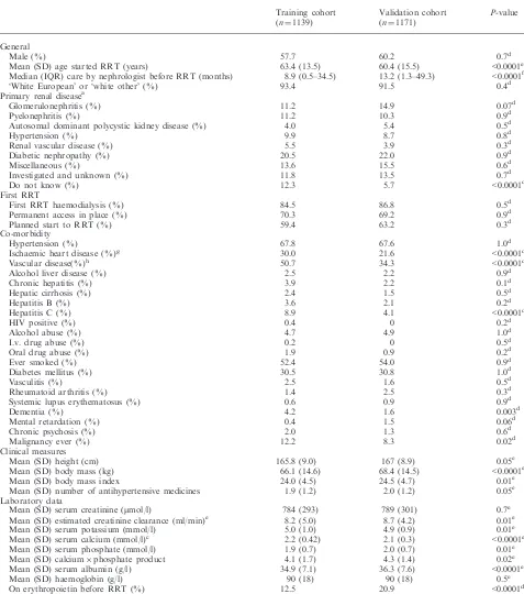
Table 1. Comparison of the baseline variables in the training and validation cohorts

Training cohort (n¼1139)

Validation cohort (n¼1171)

P-value

General

Male (%) 57.7 60.2 0.7d

Mean (SD) age started RRT (years) 63.4 (13.5) 60.4 (15.5) <0.0001e Median (IQR) care by nephrologist before RRT (months) 8.9 (0.5–34.5) 13.2 (1.3–49.3) <0.0001f

‘White European’ or ‘white other’ (%) 93.4 91.5 0.4d

Primary renal diseasea

Glomerulonephritis (%) 11.2 14.9 0.07d

Pyelonephritis (%) 11.2 10.3 0.9d

Autosomal dominant polycystic kidney disease (%) 4.0 5.4 0.5d

Hypertension (%) 9.9 8.7 0.8d

Renal vascular disease (%) 5.5 3.9 0.3d

Diabetic nephropathy (%) 20.5 22.0 0.9d

Miscellaneous (%) 13.6 15.5 0.6d

Investigated and unknown (%) 11.8 13.5 0.7d

Do not know (%) 12.3 5.7 <0.0001d

First RRT

First RRT haemodialysis (%) 84.5 86.8 0.5d

Permanent access in place (%) 70.3 69.2 0.9d

Planned start to RRT (%) 59.4 63.2 0.3d

Co-morbidity

Hypertension (%) 67.8 67.6 1.0d

Ischaemic heart disease (%)g _30.0 _21.6 _<0.0001d

Vascular disease(%)h 50.7 34.3 <0.0001d

Alcohol liver disease (%) 2.5 2.2 0.9d

Chronic hepatitis (%) 3.9 2.2 0.1d

Hepatic cirrhosis (%) 2.4 1.5 0.5d

Hepatitis B (%) 3.6 2.1 0.2d

Hepatitis C (%) 8.9 4.1 <0.0001d

HIV positive (%) 0.4 0 0.2d

Alcohol abuse (%) 4.7 4.9 1.0d

I.v. drug abuse (%) 0.2 0 0.5d

Oral drug abuse (%) 1.9 0.9 0.2d

Ever smoked (%) 52.4 54.0 0.9d

Diabetes mellitus (%) 30.5 30.8 1.0d

Vasculitis (%) 2.5 1.6 0.5d

Rheumatoid arthritis (%) 1.4 2.5 0.3d

Systemic lupus erythematosus (%) 0.6 0.9 0.9d

Dementia (%) 4.2 1.6 0.003d

Mental retardation (%) 0.4 1.5 0.06d

Chronic psychosis (%) 2.0 1.3 0.6d

Malignancy ever (%) 12.2 8.3 0.02d

Clinical measures

Mean (SD) height (cm) 165.8 (9.0) 167 (8.9) 0.05e

Mean (SD) body mass (kg) 66.1 (14.6) 68.4 (14.5) <0.0001e

Mean (SD) body mass index 24.0 (4.5) 24.5 (4.7) 0.01e

Mean (SD) number of antihypertensive medicines 1.9 (1.2) 2.0 (1.2) 0.05e Laboratory data

Mean (SD) serum creatinine (mmol/l) 784 (293) 789 (301) 0.7e

Mean (SD) estimated creatinine clearance (ml/min)e _{8.2 (5.0)} _{8.7 (4.2)} _0.01e

Mean (SD) serum potassium (mmol/l) 5.0 (1.0) 4.9 (0.9) 0.01e

Mean (SD) serum calcium (mmol/l)c _{2.2 (0.42)} _{2.1 (0.3)} _<0.0001e

Mean (SD) serum phosphate (mmol/l) 1.9 (0.7) 2.0 (0.7) 0.01e

Mean (SD) calciumphosphate product 4.1 (1.7) 4.3 (1.4) 0.02e

Mean (SD) serum albumin (g/l) 34.9 (7.1) 36.3 (7.6) <0.0001e

Mean (SD) haemoglobin (g/l) 90 (18) 90 (18) 0.5e

On erythropoietin before RRT (%) 12.5 20.9 <0.0001d

After application of Bonferroni correction for multiple comparisons, aP-value of <0.0009 was regarded as signiﬁcant for the comparison of the 58 baseline variables.

a

Grouped from ERA-EDTA PRD codes [1].

b_{Calculated using the Cockcroft and Gault formula [16].} c

Corrected for serum albumin concentration. d_t_{-test of the mean.}

e

w2test.

f_{Mann–Whitney test.}

g_{History of angina or myocardial infarction.}

h_{History of angina, myocardial infarction, cerebrovacular accident, transient ischaemic attack, symptomatic peripheral vascular disease} or arterial bypass operation.

(4)

cerebral ischaemia were combined to make ‘vascular disease’; history of malignancy, ongoing skin malignancy or ongoing non-skin malignancy were combined to make ‘malignancy ever’. Furthermore, some variables were also used to make calculated fields: ‘body mass index’, ‘estimated creatinine clearance’ (using the formula of Cockcroft and Gault [16]) and ‘calcium phosphate product’. The two groups creating the models were given exactly the same data set and the data variables were explained in detail. The teams creating the predictive models were advised that the combined or calculated fields could be used in the model if the variables used to produce them were omitted to avoid interaction of independent variables in the model (with the exception of age, gender, weight and ‘estimated creatinine clearance’). For example, it was permissible to use history of angina and history of MI in the same model but it was not permissible to use history of ischaemic heart disease and history of MI in the same model as these variables were implicitly not independent. Only three patients had renal transplant as mode of first RRT and so ‘mode of first RRT’ was re-categorized as ‘haemodialysis’ or ‘not haemodialysis’.

Serum cholesterol and parathyroid hormone (PTH) concentrations were also requested but were available for an insufﬁcient number of patients to allow meaningful analysis, and the data have not been used.

For patients starting RRT, we asked participating centres to report all patients that they considered probably had ESRF. During follow-up, we were able to identify and exclude patients who had recovered independent renal function either before or after the 90th day of RRT.

The ERA-EDTA Registry committee decided that the centres that had not participated in 1997 should be again invited to participate in February 1998. The training cohorts (i.e. patients who died on RRT in February 1997 or February 1998) have been amalgamated.

The data from the training cohort were then given to the statisticians in Amsterdam to create an MVR model and the Engineering Department at Strathclyde University, Glasgow (S.M. and M.M.) to create the self-learning RBM (see below). Each team was given exactly the same data set with known duration of survival on RRT and asked to create a model that predicts patient survival. They were then given the baseline data from patients in the validation cohort (i.e. patients who started RRT in February 1997) and asked to predict how long each patient would survive. The predictions from the two groups for the validation cohort were returned to the coordinating nephrologists and held in conﬁdence until 5-year outcome became available.

During the 6 years after inception, follow-up question-naires were sent to the centre of each patient in the validation cohort (i.e. those patients starting RRT in February 1997) after 3 and 6 months, 1, 2, 3, 4, 5 and 6 years to ask if the patient had recovered independent renal function, was alive, had died (and if so date and cause of death), was lost to follow-up or had moved centre. Patients who recovered independent renal function were excluded from further analysis. Patients who had moved centre were traced to that centre in future follow-up.

Multivariate regression (MVR) model

The time between date of start of dialysis and date of death in the training data set was modelled with a proportional hazards regression model. The hazard function and not

the density function was modelled, although there were no censored observations in this cohort. It was assumed that the risk of death attyears after start of RRT [denoted byh(t)] was a function of an unspeciﬁed baseline hazard function [h0(t)]

multiplied by a relative risk (RR) function:h(t)¼h0(t)RR.

It was assumed that the log of the relative risk was a linear function of (i) functions of observed covariate values (X1, X2,. . ., Xk); and (ii) a not-observed random region effect

(zregion): ln(RR)¼ln(zregion)þb1f1(X1)þb2f2(X2)þ

þbkfk(Xk). The random region effect was meant to

account for the effects of the different health systems, economic situations and other region-speciﬁc variables that may have affected mortality in patients from the same region and was not measured by the other covariates. It was assumed that these random effects (sometimes known as ‘frailty’ parameters) followed ag(,) distribution. The relationship between the log of the RR and each numerical covariate X[f(X)] was assessed by inspection of the marginal residuals; a linear relationship [f(X)¼X] was used if possible, and, if needed, a spline function (SAS-macro %PSPLINET) [17] was used to estimate the non-linear effect of each covariate on mortality risk. Interactions between covariates were also inspected, and violation of the assumed proportionality of each covariate was assessed by evaluating interactions between covariates and time. The cumulative baseline hazard function was modelled parametrically with a poly-nomial function of time t: H0ðtÞ ¼Rh0ðuÞdu¼aþbtþ

ct2_þ_d_t3_þ_{. For the prediction of the survival of}

the patients in the prospective cohort, the 1- and 5-year survival probabilitiesS(1) andS(5) were calculated asS(t)¼

exp[H0(t)exp[gln(RR)], wheregis a shrinkage factor.

This factor was derived from the results on the retrospective cohort, and was meant to guard against over-optimistic predictions.

Self-learning rule-based model (RBM)

The C5.0 rule induction algorithm attempts to deriveif–then prediction rules from a training data set, which can subsequently be used to classify ‘unseen’ data [18]. Rule sets and decision trees are induced by segmenting data using partitioning lines. The self-learning RBM was created using the C5.0 rule induction facilities within the Clementine software package, developed by SPSS. The rule sets were then exported and integrated within Strathclyde University’s bespoke software. The C5.0 rule induction software auto-matically identiﬁes relationships between the variables within complex data sets and creates re-usable rules. In the present application, the technique predicts outcome in groups and so the nephrologists identiﬁed survival time periods of <3, 3.01–12, 12.01–24, 24.01–59.99 and60 months as being of clinical value.

Modiﬁed Charlson score (MCS)

MCS was calculated as described recently by Hemmelgarn et al. [8] (Table 2) with adjustment for age class as in the original description [14]. The co-morbidity score is added to the age score (one additional point for each decade beginning at 40 years). ‘Disseminated malignancy’ was not speciﬁed in our questionnaire and so the only deviation we made from the MCS described in the paper by Hemmelgarnet al. was to award 5 points for history of neoplasia rather

(5)

than the 10 points for disseminated malignancy. Sensitivity analysis demonstrated that this allocation had no inﬂuence on the subsequent results presented (data not shown).

Statistical comparisons

The baseline data in the training and validation cohorts were compared byt-test of the mean, Mann–Whitney test orw2test where appropriate. After application of Bonferroni correction for multiple comparisons, aP-value of <0.001 was regarded as signiﬁcant for the comparison of the 50 baseline variables. Patient survival in the training and validation cohorts was compared by log-rank test of a Kaplan–Meier plot.

Survival predictions of the MVR model for individual patients were brought together in the same pre-deﬁned groups as the RBM (<3, 3.01–12, 12.01–24, 24.01–59.99 and 60 months). The MCSs were combined to achieve the same ﬁve predicted groups based on the MCSs in the training cohort.

The positive predictive values (PPVs) and negative predictive values (NPVs) for 1- and 5-year survival in the validation cohort were analysed to compare the utility of the models for individual patient prediction. The likelihood ratios for predicting 1- and 5-year survival were calculated, using the 1- and 5-year survival from the training cohort as the pre-test probability. The ability of the models to identify groups of patients with similar risk was compared by graphing the median and interquartile range (IQR) of the actual survival of groups of validation cohort patients predicted to survive <3, 3.01–12, 12.01–24, 24.01–59.99 and60 months.

Finally, the proportion of explained variation (PEV) for each model (i.e. how much of the total variation in survival can be explained by each model) was compared using the method of Heinze and Schemper [19].

Statistical comparative tests were performed using SPSS v10.0 (SPSS Inc., 2001) and Microsoft Excel 2002 (Microsoft Corporation, 2001).

Results

Of the 3640 dialysis centres registered with the ERA-EDTA in 1997, 1220 (33.5%) centres from 37 countries

agreed to participate in the study and either contributed patient data or indicated that no patients started RRT or died on RRT during the inception period.

A total of 1217 patient data forms were returned for patients who died during the inception period (training cohort). Of these, 66 forms contained invalid data (such as date of death outside the inception period, date of starting RRT apparently before birth, etc.), or had important missing data such as date of birth or sex. Only 12 patients were <16 years old and a decision was made to omit these from the models and apply the models only to adults. This left 1139 patients with sufﬁcient data to be used to construct the predictive models. This number includes 296 patients who started RRT in February 1998 as a result of the decision by the ERA-EDTA Registry committee that the centres that had not participated in 1997 should be again invited to participate in February 1998.

A total of 1236 patient data forms were returned for patients who had started RRT in February 1997 (validation cohort). Of these, four forms contained invalid data or had important missing data. Eighteen patients were <16 years old and were omitted. Forty-three patients recovered renal function during the follow-up period and are not included in the analysis. This left 1171 patients with sufﬁcient data to be used to validate the models.

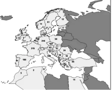
The 2310 adult patients described above, who were used to construct and validate the models, were derived from 793 centres from 37 countries in the ERA-EDTA area. The median number of patients contributed per centre was two (range 1–15) and the median number of centres per country was 12.5 with a range of 1 (Ireland, Cyprus and Malta) to 117 (Italy). The median number of patients per country was 31 with a range of 1 (Cyprus) to 338 (Italy) (Figure 2). The geographical distribution of patients in the training cohort was similar to that of the validation cohort.

Baseline data

The baseline data are shown in Table 1, with a com-parison between the training and validation cohorts. At the time of starting RRT, patients in the validation cohort were signiﬁcantly younger, had been cared for by a nephrologist for longer, were less likely to have ischaemic heart disease, vascular disease or hepatitis C infection, had a higher body mass, a lower serum calcium, a higher serum albumin, and were more likely to have been on erythropoietin before starting RRT.

Patient survival

[image:5.595.72.305.78.237.2]

By deﬁnition, survival data were available for 100% of the training cohort. For the validation cohort, 1-year survival status was available for 1021 of the 1171 patients (87.2%) and 5-year survival status for 851 patients (72.7%). In the subsequent analysis of model predictions, only patients with known survival status are included.

Table 2.Modiﬁed Charlson score (MCS) used in this study (adapted from Hemmelgarnet al. [8])

Co-morbidity variable ESRD co-morbidity weight

Myocardial infarction 2 Congestive heart failure 2 Peripheral vascular disease 1 Cerebral vascular disease 2

Dementia 1

Chronic lung disease 1

Rheumatological 1

Peptic ulcer disease 1 Diabetes without complications 2 Diabetes with complications 1

Neoplasia 5

Moderate/severe liver disease 2

Leukaemia 2

Lymphoma 5

The score for co-morbidity is added to a score for age (one additional point for each decade beginning at 40 years).

(6)

Kaplan–Meier survival curves for the two cohorts are shown in Figure 3. The survival of patients in the validation cohort was signiﬁcantly longer than in the training cohort (median survival 46.4vs 26.0 months;

P<0.0001 log rank test). The 1- and 5-year actuarial survivals in the validation cohort were 77.5 and 41.7%, respectively, compared with 69.2 and 26.5%, respec-tively, in the training cohort.

MVR model

By means of non-linear curve ﬁtting, it was found that the baseline survivor function was very well described by

S0ðtÞ ¼e½0:006þð3:88tþ35:37t2Þ=ð1þ124:7tÞ

where S0(t) is the baseline survival (the survival

proportion when all covariates are equal to zero) at a given timetsince start of RRT.

The variables included in the final model and their influences on survival are shown in Table 3. Twenty-four independent variables were included and their influences on patient survival are consistent with previously published multivariate analyses with the exceptions that history of peripheral vascular disease and hepatitis C infection were both independent predictors of longer survival. The final predictive model based on the results in Table 3 with the

incorporation of the frailty factor and theoretical shrinkage factor was:

SðtjPI;ZEÞ ¼e½0:006þð3:88tþ35:37t2Þ=ð1þ124:7tÞZEe0:93ðPI2:63Þ

where ZE is the posterior expected value of the

[image:6.595.48.408.57.348.2]

countries’ frailty estimated on the available data and PI is the prognostic index for the individual patient.

Fig. 2. Number of subjects contributed per country to either the training data set (patients on RRT who died in February 1997 or February 1998) or the validation data set (patients who started RRT in February 1997). For clarity, the ﬁgure does not include the four patients contributed from Luxembourg, the nine patients contributed from Malta and the one patient contributed from Cyprus. Countries afﬁliated to the ERA-EDTA Registry in 2004 are shown in light grey.

Fig. 3.Five-year Kaplan–Meier survival curves for the two cohorts. Numbers of patients remaining for analysis in each group (n) at each year of follow-up are shown above thex-axis.

[image:6.595.292.521.411.590.2]

(7)

RBM

After selection of different rules, the final rule was >450 lines long and is, therefore, not presented here in full. To illustrate the principle of the rule structure, however, Figure 4 provides a visual representation of one of the rule sets generated through the analysis. In that example, the starting point is age at first RRT, indicated in green. From the database, if this was unknown, then the ensuing survival rate was <3 months. If the branch for ‘age at first RRT’ >75.53 years is considered, then the next variable for classifi-cation was PTH. Depending on this measure, the subsequent variables of interest vary until a classifi-cation is achieved. The complete rule had >450 clauses within it. When applied to the validation cohort, the rule was incapable of categorizing 11 patients based on their entry data.

MCS

The range of Charlson scores was 0–15 with the median score being 4 (IQR 3–6). The MCSs in the training cohort were used to identify the previously deﬁned groups as follows: MCS 9–15 predicts survival <3 months (n¼93) in the validation cohort; MCS 6–8 predicts survival 3.01–12 months (n¼237); MCS 4–5 predicts survival 12.01–24 months (n¼251); MCS 2–3 predicts survival 24.01–59.99 months (n¼173); and MCS 0–1 predicts survival60 months (n¼97).

Comparing the three predictive models

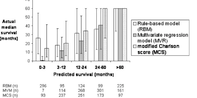
[image:7.595.73.551.68.334.2]

For predicting 1-year survival, the RBM had the highest PPV (84.2%), the MVR model had the highest NPV (47%) and the RBM had the highest likelihood ratio (1.59) (Table 4). For predicting 5-year survival, the MCS had the highest PPV (79.4%), the RBM had the highest NPV (74.3%) and the MCS had the highest likelihood ratio (7.0). In other words, 79.4% of patients with a MCS of 0 or 1 survived >5 years; 74.3% of patients predicted by the RBM to have a survival of <5 years died within 5 years; and patients who survived >5 years were seven times more likely to have an MCS of 0 or 1 than patients who died within 5 years. Figure 5 shows the comparison of the ability of the three models to discriminate groups of patients with similar risk. For the MVR model and the MCS, there is a close correlation between predicted survival and actual median survival in these pre-deﬁned groups. The IQRs are narrower in the MVR model, consistent with better discriminatory power. The RBM shows a close correlation between predicted survival and actual median survival for the groups 3–12, 12–24, 24–60 and 60 months, but the predicted survival <3 months group’s median survival was 26.1 months (IQR 7.8–54.3). The MVR model and MCS both predicted 60 month survival with precision (median survival 60 months; IQR 60–60). It should be empha-sized that the maximum possible survival in the validation cohort at the stage of the present analysis was 60 months.

Table 3. Cox proportional hazards model ﬁtted to 1139 RRT patients

Factor No. of patients Regression coefﬁcient ln(RR) RR 95% CI

Age at start of RRT (per year) – 0.05 1.05 1.04–1.05

Asian origin 26 0.71 2.02 1.33–3.08

Smoked never 311 0.16 0.85 0.74–0.98

First RRT planned (yes) 740 0.56 0.57 0.50–0.65

Serum creatinine (per 100mmol/l) – 0.04 0.96 0.94–0.98

Primary renal disease

Glomerulonephritis 127 0.03 1.03 0.80–1.34

Polycystic kidneys 45 0.31 0.73 0.51–1.04

Hypertension 113 0.16 1.17 0.89–1.53

Renal vascular disease 63 0.09 1.09 0.79–1.51

Diabetes 233 0.64 1.90 1.50–2.41

Miscellaneous 155 0.47 1.60 1.25–2.06

Investigated and unknown 134 0.11 1.12 0.87–1.45

Unknown or not recorded 140 0.31 1.36 1.06–1.76

Co-morbidities

Peripheral vascular disease 257 0.18 0.83 0.71–0.98

Myocardial infarction 166 0.29 1.33 1.12–1.59

High blood pressure 771 0.17 1.18 1.03–1.35

Cerebrovascular accident 161 0.22 1.25 1.05–1.50

Hepatitis C 101 0.42 0.66 0.53–0.82

Systemic lupus erythematosus 7 0.83 2.30 1.03–5.17

Mental retardation 4 1.75 5.77 1.90–17.55

Down syndrome 3 1.48 4.38 1.28–15.02

Malignancy ever 139 0.37 1.44 1.20–1.74

Alcohol liver disease 29 0.74 2.10 1.43–3.09

Patient on erythropoeitin (yes) 130 0.3 1.35 1.11–1.65

RR, relative risk of death. An RR of >1.0 implies the variable is independently associated with a greater hazard of death. An RR of <1.0 implies that the variable is associated with a reduced hazard of death. If the 95% conﬁdence intervals do not cross zero, then the association is statistically signiﬁcant at theP<0.05 level.

(8)

The observation in Figure 5 is consistent with the calculated PEV using the method of Heinze and Schemper. This showed that the performance of the MVR model and the MCS was similar, with a PEV of 14.6 and 12.9%, respectively, while the RBM only explained 3.95% of the total variation in survival.

Discussion

[image:8.595.59.479.76.414.2]

There have been many previous attempts to predict survival in patients starting RRT [2–8]. This study was designed in an attempt to improve on previous predictive models that were limited by the fact that

Fig. 4. (a) Representation of one branch of the rule-based model after training. Prediction of survival was made by applying the rule to the data of a patient in the validation data set. To illustrate the complexity of the model, the computer-generated text associated with this branch is shown in (b); the complete model comprises 450 clauses.

(9)

they were usually developed in a small number of patients from one geographical area, had low precision of prediction, did not include many variables that have subsequently been shown to inﬂuence survival and lacked validation in other patient populations. The large number of patients from many countries makes the results generalizable.

We also wanted to compare multiple regression modelling, the self-learning rule-based algorithm and a simple bedside scoring system. At the time the study was designed, it was being suggested that novel artificial intelligence techniques such as a self-learning rule-based algorithm may be better at predicting outcome in medicine because regression modelling was perceived to make assumptions about the input data and could not resolve relationships between independent and dependent variables that were not linear [20,21]. On the other hand, it is acknowledged that novel self-learning techniques can have limited generaliz-ability due to over-fitting to the training data set. Furthermore, refinements can be made to the MVR

technique such as testing for interactions, SPLINE functions and frailty factors, that were applied in the present study, that can overcome many of these perceived limitations. It was important to compare these sophisticated techniques with an established simple scoring system and we selected the Charlson score because it has been validated in renal patients, has a wide range of possible scores and has also recently been modiﬁed for patients on RRT [8].

[image:9.595.68.548.70.164.2]

The ambidirectional inception cohort study design is unusual. The design takes advantage of the fact that once a patient starts RRT they remain under the care of nephrologists for the remainder of their lives, with the exception of the few patients who recover renal function unexpectedly. It meant that, unlike previous studies, all of the subjects in the training cohort had reached the end-point of interest, and a prospectively followed validation cohort was included within the same study. We anticipated that, because the inception period was only 1 month, each centre would only be required to provide information on a small number of

Fig. 5.Median survival and interquartile range (to a maximum of 60 months) of patients starting RRT in February 1997 (validation cohort) according to predictions of the rule-based model (RBM), the multivariate regression (MVR) model and the modiﬁed Charlson score (MCS). Groups 1, 2, 3, 4 and 5 denote patients predicted by the RBM and MVR to survive <3, 3.01–12, 12.01–24, 24.01–59.99 and

[image:9.595.72.447.242.429.2]

60 months, respectively, and an MCS of 9–15, 6–8, 4–5, 2–3 and 0–1 (inclusive), respectively. Table 4. Comparison of model performance in predicting individual 1- and 5-year survival

Pre-test probability (%) Predicting >1 year survival (n¼1021) Predicting >5 year survival (n¼851)

69.2%a _26.5%a

MVR RBM MCSb _MVR _RBM _MCSc

PPV (%) 80.4 84.2 78.7 77.0 63.1 79.4

NPV (%) 47.0 32.6 40.8 74.2 74.3 70.2

Likelihood ratio 1.24 1.59 1.11 6.1 3.1 7.0

MVR, multivariate regression model; RBM, rule-based algorithm; MCS, modiﬁed Charlson score; PPV, positive predictive value; NPV, negative predictive value.

a_{Pre-test probability derived from the overall survival of the training cohort.} b_{MCS of <9 used as cut-off to predict survival >1 year.}

c

MCS of <2 used as cut-off to predict survival >5 years.

(10)

patients, and the case records of patients who had died while on RRT (training cohort), and patients who had started RRT (validation cohort), would be easily available to the participating nephrologists at the time of sending the questionnaires.

We anticipated that the two cohorts would be comparable, as the majority of patients in the training cohort would have started RRT within the previous 5 years when practices were similar. We were surprised to find that the patients in the validation cohort were significantly younger (mean 60.4 vs 63.4 years), had been cared for by a nephrologist for longer and were less likely to have ischaemic heart disease or vascular disease; though not surprised that they were more likely to have been on erythropoietin before starting RRT. This is not consistent with data from all renal registries that show that with time, the age and co-morbidity of patients starting RRT has increased. The baseline data and 5-year survival of the validation cohort are consistent with the EDTA-ERA Registry report for the same period [22]. There may be several reasons why patients with a high burden of co-morbidity, and hence a shorter survival, are over-represented in the training cohort. First, most of the patients in the training cohort started RRT during the period of rapidly increasing acceptance rates in Europe prior to the inception period of the study [23]. This increased acceptance rate in Europe was largely due to an increased acceptance of older patients with multiple co-morbidities. Since these were the same patients who were likely to have short survival, they are likely to be over-represented in an inception cohort of patients dying in February 1997 and February 1998 compared with a cohort of patients starting RRT in February 1997. Secondly, it is likely that some long survivors (who were young and had low co-morbidity when they started RRT), who happened to die in February 1997, are missing from the training cohort because nephrologists may not have become aware of their death until after the survey was carried out. Thirdly, reported co-morbidity may be higher because of assumptions made about co-morbidity at the time of starting RRT based on events that happened after starting RRT. Finally, the significantly better survival in the validation cohort may be partly explained by changes in practice in recent years (such as more attention to anaemia before RRT is required). Despite these differences in the training and validation cohorts, the underlying biology is likely to be the same; even if the proportions of patients with particular attributes is not the same in both groups, the risk associated with these attributes should still be contained within the data sets and the comparison of the models therefore remains valid.

Comparing predictive models is difﬁcult. The output of the MVR model is continuous, whereas the outputs of the RBM and MCS are categorical. We decided to compare the ability to predict clinically useful aspects of survival: 1- and 5-year survival. The PPV and NPV are useful statistics to quote when applying the results of the models’ predictions to individual patients.

The PPV tells the user the probability that a patient predicted by the test to survive beyond the selected time period will actually survive beyond that time period. The likelihood ratio informs about the utility of the test in the context of the pre-test survival probability. The PPVs, NPVs and likelihood ratios for predicting individual survival were broadly similar for all three predictive models but generally better for the MVR model and MCS. All three models were better at predicting 5-year than 1-year survival. The predictions of 5-year survival could be useful in the clinic setting; for example a patient with an MCS of 0 or 1 can be informed that, although the overall 5-year survival for patients starting RRT is 35.5%, the PPV of the MCS increases their probability of 5-year survival to 79.4% (Table 3). This may be used for example to support decisions regarding transplantation: in the UK, it is stipulated that expected survival of <5 years is a contra-indication to listing for cadaveric renal transplantation [24]. The utility of the MCS in predicting 5-year survival is reﬂected by the likelihood ratio of 7.0; patients who survived >5 years were seven times more likely to have an MCS of 0 or 1 than patients who died within 5 years. It has been arbitrarily suggested that a likelihood ratio of 2.0 is the minimum for utility in clinical practice [25].

All three models can identify groups of patients with different survival risk (Figure 5). All three models were able to identify a group of patients with predicted survival 60 months with sufﬁcient precision to be clinically useful, although the precision of the RBM was less than that of the other two models.

The ability to identify a group of patients with low survival might be of more value. The MVR model was able to identify a group of patients with very low (<3 months) predicted survival with useful accuracy and precision, but the prediction applied to only seven patients (0.82%) in the validation cohort. Combining the groups predicted by the MVR model to survive <3 months or 3.01–12 months into one group predicted to survive <12 months provides 121 patients (14.2%) in the validation cohort with actual median survival of 10.7 months (IQR 3–26.7). Again this would be useful when discussing transplant listing with individual patients. Furthermore, selecting patients in this way for entry into clinical trials of interventions to reduce mortality on RRT would greatly reduce the sample size required to achieve adequate statistical power. Neither the MCS nor the RBM were able to identify a similar sized group of patients with such low survival with equal precision.

There are other considerations when comparing these predictive models. The MCS is easy to apply and could be calculated quickly on paper. It is also easy to explain to a patient. The MVR model and RBM predictions require computerized calculation although with increasing use of electronic patient records there is no reason why this could not be done in the clinic setting. The clinician needs to consider how representative the patients in the study are compared with their own patients. In this respect, our study is

(11)

likely to be more representative of European dialysis patients than previous studies, but there is inevitably a bias toward the study being more representative of the countries and centres that contributed the most patients.

There are obvious reasons why the models cannot predict outcome with 100% accuracy. The first is that death is not always a direct result of the illness of interest, e.g. death in a road traffic accident. The models clearly identify co-morbid conditions as important predictors of survival, and this is consistent with all previous studies. This study and most others are limited by the fact that a co-morbid condition such as ischaemic heart disease may be present but not clinically evident and by the fact that severity of co-morbid conditions is not included. In a recent study by van Manenet al., however, adding severity of co-morbid conditions did not seem to increase the predictive power of commonly used co-morbidity indices [6]. Some factors that are likely to have a major influence on survival were included such as intravenous drug abuse but, because of the low prevalence in the training cohort, they were not identified by the models as of major importance. Finally, it is well known that clinical factors after the start of RRT, such as adequacy of dialysis [26] and renal transplant [27], influence mortality.

Conclusion

Using the ambidirectional inception cohort design of this ERA-EDTA Registry survey, we have been able to create and validate two novel instruments to predict survival in patients starting RRT. The Cox regression hazards model has become the standard for examining the relationship between independent variables and survival, and our data demonstrate the continued value. We have also validated the recently described modiﬁcation of the generic Charlson score for patients on RRT.

We have shown that these models are good at predicting long-term survival but not good at predict-ing short-term survival for individual patients. The MVR model and the MCS could, however, be used to select a group of patients at high risk of short survival.

Acknowledgements. The authors wish to express their gratitude to the representatives from the many centres who generously took the time to complete the questionnaires that made the study possible.

Conﬂict of interest statement. None declared.

References

1. ERA-EDTA Registry. ERA-EDTA Registry 2002 Annual Report. 46. Academic Medical Centre, Amsterdam, The Netherlands, 2004

2. Wright LF. Survival in patients with end-stage renal disease.

Am J Kidney Dis1991; 17: 25–28

3. Khan IH, Catto GR, Edward N, Fleming LW, Henderson IS, MacLeod AM. Inﬂuence of coexisting disease on survival on renal-replacement therapy. Lancet1993; 341: 415–418 4. Chandna SM, Schulz J, Lawrence C, Greenwood RN,

Farrington K. Is there a rationale for rationing chronic dialysis? A hospital based cohort study of factors affecting survival and morbidity.Br Med J1999; 318: 217–223 5. Davies SJ, Phillips L, Naish PF, Russell GI. Quantifying

comorbidity in peritoneal dialysis patients and its relationship to other predictors of survival. Nephrol Dial Transplant2002; 17: 1085–1092

6. van Manen JG, Korevaar JC, Dekker FW, Boeschoten EW, Bossuyt PM, Krediet RT. How to adjust for comorbidity in survival studies in ESRD patients: a comparison of different indices.Am J Kidney Dis2002; 40: 82–89

7. Miskulin DC, Martin AA, Brown R et al. Predicting 1 year mortality in an outpatient haemodialysis population: a comparison of comorbidity instruments. Nephrol Dial Transplant2004; 19: 413–420

8. Hemmelgarn BR, Manns BJ, Quan H, Ghali WA. Adapting the Charlson Comorbidity Index for use in patients with ESRD.Am J Kidney Dis2003; 42: 125–132

9. Grimes DA, Schulz KF. Cohort studies: marching towards outcomes.Lancet2002; 359: 341–345

10. Tsumoto S. Automated discovery of positive and negative knowledge in clinical databases. IEEE Eng Med Biol 2000; 19: 56–62

11. McArthur SD, Strachan SM, Jahn G. The design of a multi-agent transformer condition monitoring system. IEEE Trans Power Syst2004; 19: 1845–1852

12. John GH, Miller P, Kerber R. Stock selection using rule induction.IEEE Expert1996; 11: 52–58

13. Kahn CE. Artiﬁcial intelligence in radiology: decision support systems.Radiographics1994; 14: 849–861

14. Charlson ME, Pompei P, Ales KL, MacKenzie CR. A new method of classifying prognostic comorbidity in longitudinal studies: development and validation. J Chronic Dis 1987; 40: 373–383

15. Van Dijk PC, Jager KJ, de Charro Fet al.Renal replacement therapy in Europe: the results of a collaborative effort by the ERA-EDTA registry and six national or regional registries.

Nephrol Dial Transplant2001; 16: 1120–1129

16. Cockcroft DW, Gault MH. Prediction of creatinine clearance from the serum creatinine.Nephron1976; 16: 31–41

17. Harrell FE. Survrisk.pak with %PSPLINET MACRO. http:// biostat.mc.vanderbilt.edu/twiki/bin/view/Main/SasMacros. Accessed March 23, 2005

18. Quinlan R. C5.0 Programs for Machine Learning. Morgan Kaufmann, San Mateo, 1993

19. Heinze G, Schemper, M. RELIMPCR and RELIMPLR,

SAS-macros for the analysis of relative importance of prognostic factors in Cox and logistic regression. http:// www.akh-wien.ac.at/imc/biometrie/programme/relimp/. 2004. Accessed March 23, 2005

20. Baxt WG, Skora J. Prospective validation of artiﬁcial neural network trained to identify acute myocardial infarction.Lancet

1996; 347: 12–15

21. Dybowski R, Weller P, Chang R, Gant V. Prediction of outcome in critically ill patients using artiﬁcial neural network synthesised by genetic algorithm.Lancet1996; 347: 1146–1150 22. ERA-EDTA Registry Annual Report 1998. http:// www.era-edta-reg.org/ﬁles/annualreports/pdf/AnnRep1998.pdf. 2005. Accessed June 6, 2005

23. Stengel B, Billon S, Van Dijk PCet al. Trends in the incidence of renal replacement therapy for end-stage renal disease in Europe, 1990–1999. Nephrol Dial Transplant 2003; 18: 1824–1833

24. NHS UK Transplant. Transplant list criteria for potential renal transplant patients. http://www.uktransplant.org.uk/ukt/ about_transplants/organ_allocation/kidney_(renal)/national_

(12)

protocols_and_guidelines/protocols_and_guidelines/transplant_ list_criteria.jsp. 2003. Accessed August 28, 2005

25. Jaeschke R, Guyatt G, Sackett DL. Users’ guides to the medical literature. III. How to use an article about a diagnostic test. A. Are the results of the study valid? Evidence-Based Medicine Working Group.J Am Med Assoc1994; 271: 389–391

26. Charra B, Calemard E, Ruffet Met al. Survival as an index of adequacy of dialysis.Kidney Int1992; 41: 1286–1291 27. Wolfe RA, Ashby VB, Milford EL et al. Comparison of

mortality in all patients on dialysis, patients on dialysis awaiting transplantation, and recipients of a ﬁrst cadaveric transplant.N Engl J Med1999; 341: 1725–1730

Received for publication: 29.8.05 Accepted in revised form: 18.11.05