Muon Ionization Cooling Experiment
.
White Rose Research Online URL for this paper:
http://eprints.whiterose.ac.uk/145176/
Version: Published Version
Article:
Adams, D., Adey, D., Asfandiyarov, R. et al. (132 more authors) (2019) First
particle-by-particle measurement of emittance in the Muon Ionization Cooling Experiment.
European Physical Journal C: Particles and Fields, 79 (3). 257. ISSN 1434-6044
https://doi.org/10.1140/epjc/s10052-019-6674-y
eprints@whiterose.ac.uk https://eprints.whiterose.ac.uk/ Reuse
This article is distributed under the terms of the Creative Commons Attribution (CC BY) licence. This licence allows you to distribute, remix, tweak, and build upon the work, even commercially, as long as you credit the authors for the original work. More information and the full terms of the licence here:
https://creativecommons.org/licenses/
Takedown
If you consider content in White Rose Research Online to be in breach of UK law, please notify us by
https://doi.org/10.1140/epjc/s10052-019-6674-y
Regular Article - Experimental Physics
First particle-by-particle measurement of emittance in the Muon
Ionization Cooling Experiment
MICE Collaboration
D. Adams15, D. Adey25,34, R. Asfandiyarov13, G. Barber18, A. de Bari6, R. Bayes16, V. Bayliss15, R. Bertoni4, V. Blackmore18,a, A. Blondel13, J. Boehm15, M. Bogomilov1, M. Bonesini4, C. N. Booth20, D. Bowring25, S. Boyd22, T. W. Bradshaw15, A. D. Bross25, C. Brown15,23, G. Charnley14, G. T. Chatzitheodoridis16,21, F. Chignoli4,
M. Chung10, D. Cline30, J. H. Cobb19, D. Colling18, N. Collomb14, P. Cooke17, M. Courthold15, L. M. Cremaldi28, A. DeMello26, A. J. Dick21, A. Dobbs18, P. Dornan18, F. Drielsma13, K. Dumbell14, M. Ellis23, F. Filthaut11,32, P. Franchini22, B. Freemire27, A. Gallagher14, R. Gamet17, R. B. S. Gardener23, S. Gourlay26, A. Grant14, J. R. Greis22, S. Griffiths14, P. Hanlet27, G. G. Hanson29, T. Hartnett14, C. Heidt29, P. Hodgson20, C. Hunt18, S. Ishimoto9, D. Jokovic12, P. B. Jurj18, D. M. Kaplan27, Y. Karadzhov13, A. Klier29, Y. Kuno8, A. Kurup18, P. Kyberd23, J-B. Lagrange18, J. Langlands20, W. Lau19, D. Li26, Z. Li3, A. Liu25, K. Long18, T. Lord22, C. Macwaters15, D. Maletic12, B. Martlew14, J. Martyniak18, R. Mazza4, S. Middleton18, T. A. Mohayai27, A. Moss14, A. Muir14, I. Mullacrane14, J. J. Nebrensky23, D. Neuffer25, A. Nichols15, J. C. Nugent16, A. Oates14, D. Orestano7, E. Overton20, P. Owens14, V. Palladino5, M. Palmer24, J. Pasternak18, V. Pec20, C. Pidcott22,33, M. Popovic25, R. Preece15, S. Prestemon26, D. Rajaram27, S. Ricciardi15, M. Robinson20, C. Rogers15, K. Ronald21, P. Rubinov25, H. Sakamoto8,31, D. A. Sanders28, A. Sato8, M. Savic12, P. Snopok27, P. J. Smith20, F. J. P. Soler16, Y. Song2, T. Stanley15, G. Stokes14, V. Suezaki27, D. J. Summers28, C. K. Sung10, J. Tang2, J. Tarrant15, I. Taylor22, L. Tortora7, Y. Torun27, R. Tsenov1, M. Tucker14, M. A. Uchida18, S. Virostek26, G. Vankova-Kirilova1,
P. Warburton14, S. Wilbur20, A. Wilson15, H. Witte24, C. White14, C. G. Whyte21, X. Yang30, A. R. Young21, M. Zisman26
1Department of Atomic Physics, St. Kliment Ohridski University of Sofia, Sofia, Bulgaria 2Institute of High Energy Physics, Chinese Academy of Sciences, Beijing, China 3Sichuan University, Chengdu, China
4Dipartimento di Fisica G. Occhialini, Sezione INFN Milano Bicocca, Milan, Italy
5Sezione INFN Napoli and Dipartimento di Fisica, Università Federico II, Complesso Universitario di Monte S. Angelo, Naples, Italy 6Sezione INFN Pavia and Dipartimento di Fisica, Pavia, Italy
7INFN Sezione di Roma Tre and Dipartimento di Matematica e Fisica, Università Roma Tre, Rome, Italy 8Department of Physics, Graduate School of Science, Osaka University, Toyonaka, Osaka, Japan
9High Energy Accelerator Research Organization (KEK), Institute of Particle and Nuclear Studies, Tsukuba, Ibaraki, Japan 10UNIST, Ulsan, Korea
11Nikhef, Amsterdam, The Netherlands
12Institute of Physics, University of Belgrade, Belgrade, Serbia
13DPNC, Section de Physique, Université de Genève, Geneva, Switzerland 14STFC Daresbury Laboratory, Daresbury, Cheshire, UK
15STFC Rutherford Appleton Laboratory, Harwell Oxford, Didcot, UK
16School of Physics and Astronomy, The University of Glasgow, Kelvin Building, Glasgow, UK 17Department of Physics, University of Liverpool, Liverpool, UK
18Blackett Laboratory, Department of Physics, Imperial College London, London, UK 19Department of Physics, University of Oxford, Denys Wilkinson Building, Oxford, UK 20Department of Physics and Astronomy, University of Sheffield, Sheffield, UK 21SUPA and the Department of Physics, University of Strathclyde, Glasgow, UK 22Department of Physics, University of Warwick, Coventry, UK
23Brunel University, Uxbridge, UK
24Brookhaven National Laboratory, Upton, NY, USA 25Fermilab, Batavia, IL, USA
26Lawrence Berkeley National Laboratory, Berkeley, CA, USA 27Illinois Institute of Technology, Chicago, IL, USA
30University of California, Los Angeles, CA, USA 31Current address:RIKEN, Wako, Japan
32Also atRadboud University, Nijmegen, The Netherlands
33Current address:Department of Physics and Astronomy, University of Sheffield, Sheffield, UK 34Current address:Institute of High Energy Physics, Chinese Academy of Sciences, Bejing, China
Received: 31 October 2018 / Accepted: 11 February 2019 / Published online: 21 March 2019 © The Author(s) 2019
Abstract The Muon Ionization Cooling Experiment (MICE) collaboration seeks to demonstrate the feasibility of ionization cooling, the technique by which it is proposed to cool the muon beam at a future neutrino factory or muon collider. The emittance is measured from an ensemble of muons assembled from those that pass through the experi-ment. A pure muon ensemble is selected using a particle-identification system that can reject efficiently both pions and electrons. The position and momentum of each muon are measured using a high-precision scintillating-fibre tracker in a 4 T solenoidal magnetic field. This paper presents the tech-niques used to reconstruct the phase-space distributions in the upstream tracking detector and reports the first particle-by-particle measurement of the emittance of the MICE Muon Beam as a function of muon-beam momentum.
1 Introduction
Stored muon beams have been proposed as the source of neutrinos at a neutrino factory [1,2] and as the means to deliver multi-TeV lepton-antilepton collisions at a muon col-lider [3,4]. In such facilities the muon beam is produced from the decay of pions generated by a high-power pro-ton beam striking a target. The tertiary muon beam occu-pies a large volume in phase space. To optimise the muon yield for a neutrino factory, and luminosity for a muon col-lider, while maintaining a suitably small aperture in the muon-acceleration system requires that the muon beam be ‘cooled’ (i.e., its phase-space volume reduced) prior to acceleration. An alternative approach to the production of low-emittance muon beams through the capture ofµ+µ− pairs close to threshold in electron–positron annihilation has recently been proposed [5]. To realise the luminosity required for a muon collider using this scheme requires the substantial challenges presented by the accumulation and acceleration of the intense positron beam, the high-power muon-production target, and the muon-capture system to be addressed.
D. Cline, M. Zisman: Deceased.
ae-mail:v.blackmore@imperial.ac.uk
A muon is short-lived, with a lifetime of 2.2µs in its rest frame. Beam manipulation at low energy (≤ 1 GeV) must be carried out rapidly. Four cooling techniques are in use at particle accelerators: synchrotron-radiation cooling [6]; laser cooling [7–9]; stochastic cooling [10]; and electron cool-ing [11]. In each case, the time taken to cool the beam is long compared to the muon lifetime. In contrast, ionization cooling is a process that occurs on a short timescale. A muon beam passes through a material (the absorber), loses energy, and is then re-accelerated. This cools the beam efficiently with modest decay losses. Ionization cooling is therefore the technique by which it is proposed to increase the number of particles within the downstream acceptance for a neu-trino factory, and the phase-space density for a muon col-lider [12–14]. This technique has never been demonstrated experimentally and such a demonstration is essential for the development of future high-brightness muon accelerators or intense muon facilities.
The international Muon Ionization Cooling Experiment (MICE) has been designed [15] to perform a full demon-stration of transverse ionization cooling. Intensity effects are negligible for most of the cooling channels conceived for the neutrino factory or muon collider [16]. This allows the MICE experiment to record muon trajectories one particle at a time. The MICE collaboration has constructed two solenoidal spectrometers, one placed upstream, the other downstream, of the cooling cell. An ensemble of muon trajectories is assembled offline, selecting an initial distribution based on quantities measured in the upstream particle-identification detectors and upstream spectrometer. This paper describes the techniques used to reconstruct the phase-space distribu-tions in the spectrometers. It presents the first measurement of the emittance of momentum-selected muon ensembles in the upstream spectrometer.
2 Calculation of emittance
A beam travelling through a portion of an accelerator may be described as an ensemble of particles. Consider a beam that propagates in the positivezdirection of a right-handed Cartesian coordinate system,(x,y,z). The position of the
ith particle in the ensemble is ri = (xi,yi)and its
trans-verse momentum ispT i = (pxi,pyi); ri and pT i define
the coordinates of the particle in transverse phase space. The normalised transverse emittance,εN, of the ensemble
approximates the volume occupied by the particles in four-dimensional phase space and is given by
εN =
1
mµ
4 √
detC, (1)
where mµ is the rest mass of the muon, C is the
four-dimensional covariance matrix,
C=
⎛
⎜ ⎜ ⎝
σx x σx px σx y σx py
σx px σpxpx σypx σpxpy
σx y σypx σyy σypy
σx py σpxpy σypy σpypy ⎞
⎟ ⎟ ⎠
, (2)
andσαβ, whereα, β=x,y,px,py, is given by
σαβ=
1
N−1
ΣiNαiβi−
ΣiNαi ΣiNβi N
, (3)
andNis the number of muons in the ensemble.
The MICE experiment was operated such that muons passed through the experiment one at a time. The phase-space coordinates of each muon were measured. An ensem-ble of muons that was representative of the muon beam was assembled using the measured coordinates. The normalised transverse emittance of the ensemble was then calculated by evaluating the sums necessary to construct the covariance matrix,C, and using Eq.1.
3 The Muon Ionization Cooling Experiment
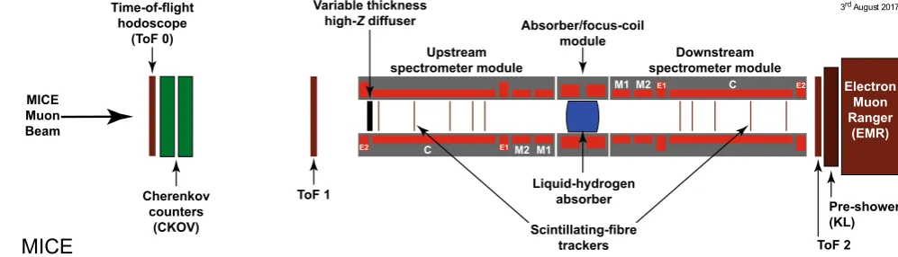
The muons for MICE came from the decay of pions pro-duced by an internal target dipping directly into the circulat-ing proton beam of the ISIS synchrotron at the Rutherford Appleton Laboratory (RAL) [18,19]. The burst of particles resulting from one target dip is referred to as a ‘spill’. A transfer line of nine quadrupoles, two dipoles and a super-conducting ‘decay solenoid’ selected a momentum bite and transported the beam into the experiment [20]. The small fraction of pions that remained in the beam were rejected during analysis using the time-of-flight hodoscopes, TOF0 and TOF1, and Cherenkov counters that were installed in the MICE Muon Beam line upstream of the cooling experi-ment [21,22]. A ‘diffuser’ was installed at the upstream end of the experiment to vary the initial emittance of the beam by introducing a changeable amount of tungsten and brass, which are high-Z materials, into the beam path [20].
A schematic diagram of the experiment is shown in Fig. 1. It contained an absorber/focus-coil module sand-wiched between two spectrometer-solenoid modules that provided a uniform magnetic field for momentum mea-surement. The focus-coil module had two separate wind-ings that were operated with the same, or opposed, polar-ities. A lithium-hydride or liquid-hydrogen absorber was placed at the centre of the focus-coil module. An iron Par-tial Return Yoke (PRY) was installed around the experiment to contain the field produced by the solenoidal spectrom-eters (not shown in Fig. 1). The PRY was installed at a distance from the beam axis such that its effect on the tra-jectories of particles travelling through the experiment was negligible.
The emittance was measured upstream and downstream of the absorber and focus-coil module using scintillating-fibre tracking detectors [26] immersed in the solenoidal field pro-vided by three superconducting coils E1, C, and E2. The
Fig. 1 Schematic diagram of the MICE experiment. The red rectangles represent the coils of the spectrometer solenoids and focus-coil mod-ule. The individual coils of the spectrometer solenoids are labelled E1, C, E2, M1 and M2. The various detectors (time-of-flight hodoscopes
[image:4.595.41.540.525.668.2](b) (a)
Fig. 2 aTop and bside views of the MICE Muon Beam line, its instrumentation, and the experimental configuration. A titanium tar-get dipped into the ISIS proton synchrotron and the resultant spill of particles was captured with a quadrupole triplet (Q1–3) and transported
through momentum-selecting dipoles (D1, D2). The quadrupole triplets (Q4–6, Q7–9) transported particles to the upstream spectrometer mod-ule. The time-of-flight of particles, measured between TOF0 and TOF1, was used for particle identification
trackers were used to reconstruct the trajectories of indi-vidual muons at the entrance and exit of the absorber. The trackers were each constructed from five planar stations of scintillating fibres, each with an active radius of 150 mm. The track parameters were reported at the nominal reference plane: the surface of the scintillating-fibre plane closest to the absorber [30]. Hall probes were installed on the tracker to measure the magnetic-field strength in situ. The instrumen-tation up- and downstream of the spectrometer modules was used to select a pure sample of muons. The reconstructed tracks of the selected muons were then used to measure the muon-beam emittance at the upstream and downstream tracker reference planes. The spectrometer-solenoid modules also contained two superconducting ‘matching’ coils (M1, M2) that were used to match the optics between the uniform-field region and the neighbouring focus-coil module. The MICE coordinate system is such that thezaxis is coincident with the beam direction, theyaxis points vertically upward, and thexaxis completes a right-handed co-ordinate system. This paper discusses the measurement of emittance using only the tracker and beam-line instrumentation upstream of the absorber. The diffuser was fully retracted for the data presented here, i.e. no extra material was introduced into the centre of the beam line, so that the incident particle distribu-tion could be assessed.
4 MICE Muon beam line
The MICE Muon Beam line is shown schematically in Fig.2. It was capable of delivering beams with normalised transverse emittance in the range 3 εN 10 mm and
mean momentum in the range 140 pµ 240 MeV/c
with a root-mean-squared (RMS) momentum spread of ∼
20 MeV/c[20] after the diffuser (Fig.1).
Pions produced by the momentary insertion of a titanium target [18,19] into the ISIS proton beam were captured using a quadrupole triplet (Q1–3) and transported to a first dipole magnet (D1), which selected particles of a desired momen-tum bite into the 5 T decay solenoid (DS). Muons produced in pion decay in the DS were momentum-selected using a second dipole magnet (D2) and focused onto the diffuser by a quadrupole channel (Q4–6 and Q7–9). In positive-beam running, a borated polyethylene absorber of variable thick-ness was inserted into the beam just downstream of the decay solenoid to suppress the high rate of protons that were pro-duced at the target [31].
muons in the pion rest frame. This produced an almost pure muon beam.
Data were taken in October 2015 in muon mode at a nominal momentum of 200 MeV/c, with ISIS in opera-tion at 700 MeV. These data [32] are used here to charac-terise the properties of the beam accepted by the upstream solenoid with all diffuser irises withdrawn from the beam. The upstream E1-C-E2 coils in the spectrometer module were energised and produced a field of 4 T, effectively uniform across the tracking region, while all other coils were unpow-ered. Positively charged particles were selected due to their higher production rate in 700 MeV proton-nucleus collisions.
5 Simulation
Monte Carlo simulations were used to determine the accuracy of the kinematic reconstruction, to evaluate the efficiency of the response of the scintillating-fibre tracker, and to study systematic uncertainties. A sufficient number of events were generated to ensure that statistical uncertainties from the sim-ulations were negligible in comparison to those of the data.
The beam impinging on TOF0 was modelled using G4beamline [33]. Particles were produced at the target using a parameterised particle-production model. These particles were tracked through the MICE Muon Beam line taking into account all material in and surrounding the beam line and using realistic models of the fields and apertures of the vari-ous magnets. The G4beamline simulation was tuned to repro-duce the observed particle distributions at TOF0.
The MICE Analysis User Software (MAUS) [34] pack-age was used to simulate the passpack-age of particles from TOF0 through the remainder of the MICE Muon Beam line and through the solenoidal lattice. This simulation includes the response of the instrumentation and used the input distribu-tion produced using G4beamline. MAUS was also used for offline reconstruction and to provide fast real-time detector reconstruction and data visualisation during MICE running. MAUS uses GEANT4 [35,36] for beam propagation and the simulation of detector response. ROOT [37] was used for data visualisation and for data storage. The particles gener-ated were subjected to the same trigger requirements as the data and processed by the same reconstruction programs.
6 Beam selection
Data were buffered in the front-end electronics and read out at the end of each spill [20]. For the reconstructed data presented here, the digitisation of analogue signals received from the detectors was triggered by a coincidence of signals in the PMTs serving a single scintillator slab in TOF1. Any slab in TOF1 could generate a trigger.
The following cuts were used to select muons passing through the upstream tracker:
– One reconstructed space-point in TOF0 and TOF1 Each TOF hodoscope was composed of two perpendicular planes of scintillator slabs arranged to measure thexand
ycoordinates. A space-point was formed from the inter-section of hits in thex andy projections. Figure3a, b show the hit multiplicity in TOF0 plotted against the hit multiplicity in TOF1 for reconstructed data and recon-structed Monte Carlo respectively. The sample is domi-nated by events with one space-point in both TOF0 and TOF1. This cut removes events in which two particles enter the experiment within the trigger window.
– Relative time-of-flight between TOF0 and TOF1, trel,in the range1 ≤ trel ≤ 6ns The time of flight between TOF0 and TOF1,t01, was measured relative to the mean positron time of flight,te. Figure3c shows the relative
time-of-flight distribution in data (black, circles) and sim-ulation (filled histogram). All cuts other than the relative time-of-flight cut have been applied in this figure. The time-of-flight of particles relative to the mean positron time-of-flight is calculated as
trel=t01−(te+δte) ,
whereδteaccounts for the difference in transit time, or
path length travelled, between electrons and muons in the field of the quadrupole triplets [21]. This cut removes electrons from the selected ensemble as well as a small number of pions. The data has a longer tail compared to the simulation, which is related to the imperfect simu-lation of the longitudinal momentum of particles in the beam (see Sect.7.1).
– A single track reconstructed in the upstream tracker with a track-fitχ2satisfying Nχ2
DOF ≤4 NDOF is the number
of degrees of freedom. The distribution ofNχ2
DOF is shown
in Fig.3d. This cut removes events with poorly recon-structed tracks. Multi-track events, in which more than one particle passes through the same pixel in TOF0 and TOF1 during the trigger window, are rare and are also removed by this cut. The distribution of Nχ2
DOF is broader
and peaked at slightly larger values in the data than in the simulation.
– Track contained within the fiducial volume of the tracker
(a) (b)
(d) (e)
(c)
Fig. 3 Distribution of the quantities that were used to select the sample used to reconstruct the emittance of the beam:athe number of space-points in TOF0 plotted against the number of space-space-points in TOF1 for reconstructed data, andbreconstructed simulation;cdistribution of the relative time-of-flight,trel;ddistribution of χ
2
NDOF; andedistribution
ofRdiff. The 1D distributions show reconstructed data as solid (black)
circles and reconstructed MAUS simulation as the solid (yellow) his-togram. The solid (black) lines indicate the position of the cuts made on these quantities. Events enter these plots if all cuts other than the cut under examination are passed
– Extrapolated track radius at the diffuser, Rdiff ≤90mm Muons that pass through the annulus of the diffuser, which includes the retracted irises, lose a substantial amount of energy. Such muons may re-enter the
[image:7.595.53.538.51.578.2](a) (b)
Fig. 4 Time of flight between TOF0 and TOF1 (t01) plotted as a
func-tion of the muon momentum,p, measured in the upstream tracker. All cuts other than the muon hypothesis have been applied. Particles within the black lines are selected. The white dotted line is the trajectory of
[image:8.595.298.510.56.233.2]a muon that loses the most probable momentum (20 MeV/c) between TOF1 and the tracker inareconstructed data, andbreconstructed Monte Carlo
Table 1 The number of particles that pass each selection criterion. A total of 24,660 particles pass all of the cuts
Cut No. surviving
particles
Cumulative surviving particles
None 53 276 53 276
One space-point in TOF0 and TOF1 37 619 37 619
Relative time of flight in range 1–6 ns 37 093 36 658
Single reconstructed track with Nχ2
DOF ≤4 40 110 30 132
Track within fiducial volume of tracker 52 039 29 714 Extrapolated track radius at diffuser≤ 90 mm 42 592 25 310
Muon hypothesis 34 121 24 660
All 24 660 24 660
into the experiment. Back-extrapolation of tracks to the exit of the diffuser yields a measurement of Rdiff with a resolution ofσRdiff =1.7 mm. Figure3e shows the
dis-tribution ofRdiff, where the difference between data and simulation lies above the accepted radius. These differ-ences are due to approximations in modelling the outer material of the diffuser. The cut onRdiffaccepts particles that passed at least 5.9σRdiff inside the aperture limit of
the diffuser.
– Particle consistent with muon hypothesisFigure4shows
t01, the time-of-flight between TOF0 and TOF1, plotted as a function of p, the momentum reconstructed by the upstream tracking detector. Momentum is lost between TOF1 and the reference plane of the tracker in the mate-rial of the detectors. A muon that loses the most proba-ble momentum,∆p ≃ 20 MeV/c, is shown as the dot-ted (white) line. Particles that are poorly reconstrucdot-ted, or have passed through support material upstream of the tracker and have lost significant momentum, are excluded
by the lower bound. The population of events above the upper bound are ascribed to the passage of pions, or mis-reconstructed muons, and are also removed from the anal-ysis.
A total of 24,660 events pass the cuts listed above. Table1
shows the number of particles that survive each individ-ual cut. Data distributions are compared to the distributions obtained using the MAUS simulation in Figs.3and4. Despite minor disagreements, the agreement between the simulation and data is sufficiently good to give confidence that a clean sample of muons has been selected.
The expected pion contamination of the unselected ensem-ble of particles has been measured to be≤0.4 %[22]. Table2
[image:8.595.174.544.308.448.2]Table 2 The number of reconstructed electrons, muons, and pions at the upstream tracker that survive each cut in the Monte Carlo simulation. Application of all cuts removes almost all positrons and pions in the reconstructed Monte Carlo sample. In the Monte Carlo simulation, a total of 253,504 particles pass all of the cuts described in the text
Cut e µ π Total
None 14,912 432,294 1610 463,451
One space-point in TOF0 and TOF1 11,222 353,613 1213 376,528 Relative Time of flight in range 1–6 ns 757 369,337 1217 379,761
Single reconstructed track with NχDOF2 ≤4 10,519 407,276 1380 419,208 Track within fiducial volume of tracker 14,527 412,857 1427 443,431 Tracked radius at diffuser≤90 mm 11,753 311,076 856 334,216 Muon hypothesis (above lower limit) 3225 362,606 411 367,340 Muon hypothesis (below upper limit) 12,464 411,283 379 424,203
Muon hypothesis (overall) 2724 358,427 371 361,576
All 22 253,475 5 253,504
7 Results
7.1 Phase-space projections
The distributions of x,y,px,py,pz, and p =
p2
x +p2y+p2z are shown in Fig.5. The total momentum
of the muons that make up the beam lie within the range 140 |p| 260 MeV/c. The results of the MAUS sim-ulation, which are also shown in Fig.5, give a reasonable description of the data. In the case of the longitudinal com-ponent of momentum, pz, the data are peaked to slightly
larger values than the simulation. The difference is small and is reflected in the distribution of the total momentum,
p. As the simulation began with particle production from the titanium target, any difference between the simulated and observed particle distributions would be apparent in the mea-sured longitudinal and total momentum distributions. The scale of the observed disagreement is small, and as such the simulation adequately describes the experiment. The dis-tributions of the components of the transverse phase space (x,px,y,py) are well described by the simulation.
Nor-malised transverse emittance is calculated with respect to the means of the distributions (Eq.2), and so is unaffected by this discrepancy.
The phase space occupied by the selected beam is shown in Fig.6. The distributions are plotted at the reference sur-face of the upstream tracker. The beam is moderately well centred in the (x,y) plane. Correlations are apparent that couple the position and momentum components in the trans-verse plane. The transtrans-verse position and momentum coordi-nates are also seen to be correlated with total momentum. The correlation in the(x,py) and(y,px)plane is due to
the solenoidal field, and is of the expected order. The disper-sion and chromaticity of the beam are discussed further in Sect.7.2.
7.2 Effect of dispersion, chromaticity, and binning in longitudinal momentum
Momentum selection at D2 introduces a correlation, dis-persion, between the position and momentum of particles. Figure 7 shows the transverse position and momentum with respect to the total momentum, p, as measured at the upstream-tracker reference plane. Correlations exist between all four transverse phase-space co-ordinates and the total momentum.
Emittance is calculated in 10 MeV/cbins of total momen-tum in the range 185 ≤ p ≤ 255 MeV/c. This bin size was chosen as it is commensurate with the detector reso-lution. Calculating the emittance in momentum increments makes the effect of the optical mismatch, or chromaticity, small compared to the statistical uncertainty. The range of 185≤ p≤255 MeV/cwas chosen to maximise the number of particles in each bin that are not scraped by the aperture of the diffuser.
7.3 Uncertainties on emittance measurement
7.3.1 Statistical uncertainties
The statistical uncertainty on the emittance in each momen-tum bin is calculated asσε = √ε
2N [38–40], whereεis the
emittance of the ensemble of muons in the specified momen-tum range and N is the number of muons in that ensem-ble. The number of events per bin varies from∼ 4 000 for
p∼190 MeV/cto∼700 forp∼250 MeV/c.
7.4 Systematic uncertainties
7.4.1 Uncorrelated systematic uncertainties
correspond-(a) (b)
(d)
(e) (f)
(c)
Fig. 5 Position and momentum distributions of muons reconstructed at the reference surface of the upstream tracker:ax,by,cpx,dpy,epz,
andf p, the total momentum. The data are shown as the solid circles while the results of the MAUS simulation are shown as the yellow histogram
ing to the RMS resolution of the quantity in question. The emittance of the ensembles selected with the changed cut values were calculated and compared to the emittance calcu-lated using the nominal cut values and the difference taken as the uncertainty due to changing the cut boundaries. The overall uncertainty due to beam selection is summarised in Table3. The dominant beam-selection uncertainty is in the
selection of particles that successfully pass within the inner 90 mm of the diffuser aperture.
[image:10.595.57.541.57.568.2](a) (b)
(c) (d)
(e) (f)
Fig. 6 Transverse phase space occupied by selected muons transported through the MICE Muon Beam line to the reference plane of the upstream tracker.a(x,px),b(x,py).c(y,px),d(y,py).e(x,y), andf(px,py)
from the nominal emittance were added in quadrature sep-arately to obtain the total positive and negative systematic uncertainty. Sources of correlated uncertainties are discussed below.
7.4.2 Correlated systematic uncertainties
[image:11.595.77.517.52.567.2](a)
(b)
(c)
(d)
Fig. 7 The effect of dispersion, the dependence of the components of transverse phase space on the momentum,p, is shown at the reference surface of the upstream tracker:a)(x,p);b(px,p);c(y,p);d(py,p)
momentum of each muon to fluctuate around its measured value according to a Gaussian distribution of width equal to
the measurement uncertainty onp. In Table3this uncertainty is listed as ‘Binning inp’.
A second uncertainty that is correlated with total momen-tum is the uncertainty on the reconstructedx,px,y, andpy.
The effect on the emittance was evaluated with the same pro-cedure used to evaluate the uncertainty due to binning in total momentum. This is listed as ‘Tracker resolution’ in Table3. Systematic uncertainties correlated with p are primarily due to the differences between the model of the apparatus used in the reconstruction and the hardware actually used in the experiment. The most significant contribution arises from the magnetic field within the tracking volume. Parti-cle tracks are reconstructed assuming a uniform solenoidal field, with no fringe-field effects. Small non-uniformities in the magnetic field in the tracking volume will result in a disagreement between the true parameters and the recon-structed values. To quantify this effect, six field models (one optimal and five additional models) were used to estimate the deviation in reconstructed emittance from the true value under realistic conditions. Three families of field model were investigated, corresponding to the three key field descriptors: field scale, field alignment, and field uniformity. The values of these descriptors that best describe the Hall-probe mea-surements were used to define the optimal model and the uncertainty in the descriptor values were used to determine the 1σvariations.
7.4.3 Field scale
Hall-probes located on the tracker provided measurements of the magnetic field strength within the tracking volume at known positions. An optimal field model was produced with a scale factor of 0.49 % that reproduced the Hall-probe measurements. Two additional field models were produced which used scale factors that were one standard deviation,
±0.03 %, above and below the nominal value.
7.4.4 Field alignment
A field-alignment algorithm was developed based on the determination of the orientation of the field with respect to the mechanical axis of the tracker using coaxial tracks with
pT ≈0 [41]. The field was rotated with respect to the tracker
by 1.4±0.1 mrad about thexaxis and 0.3±0.1 mrad about the y axis. The optimal field model was created such that the simulated alignment is in agreement with the measure-ments. Two additional models that vary the alignment by one standard deviation were also produced.
7.4.5 Field uniformity
[image:12.595.77.258.49.622.2]P
age 12 of 15
Eur
.
Ph
ys.
J.
C
(2019)
[image:13.595.79.738.130.477.2]79 :257
Table 3 Emittance together with the statistical and systematic uncertainties and biases as a function of mean total momentum,p
Source p(MeV/c)
190 200 210 220 230 240 250
Measured emittance (mm rad) 3.40 3.65 3.69 3.65 3.69 3.62 3.31 Statistical uncertainty ±3.8×10⁻²
±4.4×10⁻²
±5.0×10⁻²
±5.8×10⁻²
±7.0×10⁻²
±8.4×10⁻²
±9.2×10⁻² Beam selection:
Diffuser aperture 4.9×10⁻² 5.3
×10−2 4.9
×10−2 4.7
×10−2 4.2
×10−2 11.0
×10−2 4.4
×10−2
−3.5×10⁻²
−5.1×10⁻²
−5.7×10⁻²
−5.0×10⁻²
−3.5×10⁻²
−5.0×10⁻²
−9.6×10⁻² χ2
NDOF ≤4 5.1×10
−3 2.0
×10−3 1.0×10⁻² 4.1×10⁻³ 1.2×10⁻³ 5.5×10⁻³ 7.9×10⁻³ −4.8×10⁻³
−1.3×10⁻³
−1.8×10⁻³
−3.3×10⁻³
−2.8×10⁻⁴
−6.5×10⁻³
−4.7×10⁻⁴ Muon hypothesis 4.5×10⁻³ 2.2
×10−4 6.4
×10−3 3.1
×10−3 1.4
×10−3 2.6
×10−3 1.3
×10−3
−3.2×10⁻³ −6.8×10⁻³ −8.8×10⁻⁴ −4.7×10⁻³ −1.1×10⁻² −6.7×10⁻² −4.1×10⁻³ Beam selection (Overall) 4.9×10⁻² 5.3×10⁻² 5.0×10⁻² 4.7×10⁻² 4.2×10⁻² 1.1×10⁻¹ 4.5×10⁻²
−3.6×10⁻² −5.2×10⁻² −5.8×10⁻² −5.0×10⁻² −3.9×10⁻² −8.4×10⁻² −9.6×10⁻² Binning inp ±1.8×10⁻² ±2.1×10⁻² ±2.3×10⁻² ±2.9×10⁻² ±3.5×10⁻² ±4.3×10⁻² ±5.2×10⁻² Magnetic field misalignment and scale:
Bias −1.3×10⁻² −1.4×10⁻² −1.5×10⁻² −1.6×10⁻² −1.6×10⁻² −1.7×10⁻² −1.6×10⁻² Uncertainty ±2.0×10⁻⁴ ±2.9×10⁻⁴ ±8.0×10⁻⁴ ±4.8×10⁻⁴ ±5.5×10⁻⁴ ±4.8×10⁻⁴ ±4.9×10⁻⁴ Tracker resolution ±1.6×10⁻³
±2.1×10⁻³
±2.8×10⁻³
±3.8×10⁻³
±5.3×10⁻³
±7.0×10⁻³
±9.5×10⁻³ Total systematic uncertainty 5.2×10⁻² 5.7
×10−2 5.5
×10−2 5.6
×10−2 5.5
×10−2 11.7
×10−2 6.9
×10−2
−4.0×10⁻²
−5.6×10⁻²
−6.2×10⁻²
−5.8×10⁻²
−5.2×10⁻²
−9.5×10⁻²
−11.0×10⁻² Corrected emittance (mm rad) 3.41 3.66 3.71 3.67 3.71 3.65 3.34
Total uncertainty ±0.06 ±0.07 +0.07 ±0.08 ±0.09 +0.14 +0.12
−0.08 −0.13 −0.14
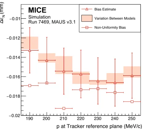
Fig. 8 The systematic bias and uncertainty on the reconstructed emit-tance under different magnetic field model assumptions. The bias esti-mate (open triangles) includes the non-uniformity bias (open squares). The variation between the models (see text) is indicated by the shaded bands
using the ‘as-built’ parameters and the partial return yoke. A simple field model was created using only the individual coil geometries to provide additional information on the effect of field uniformity on the reconstruction. The values for the sim-ple field model were normalised to the Hall-probe measure-ments as for the other field models. This represents a signif-icant deviation from the COMSOL model, but demonstrates the stability of the reconstruction with respect to changes in field uniformity, as the variation in emittance between all field models is small (less than 0.002 mm).
For each of the 5 field models, multiple 2000-muon ensembles were generated for each momentum bin. The devi-ation of the calculated emittance from the true emittance was found for each ensemble. The distribution of the dif-ference between the ensemble emittance and the true emit-tance was assumed to be Gaussian with meanεand variance
s2=σ2+θ2, whereσ is the statistical uncertainty andθis an additional systematic uncertainty. The systematic bias for each momentum bin was then calculated as [43]
∆εN = ε −εtrue, (4)
where εtrue is the true beam emittance in that momentum bin andεis the mean emittance from the N ensembles. The systematic uncertainty was calculated assuming that the distribution of residuals ofεi from the mean,ε, satisfies a
χ2distribution withN−1 degrees of freedom,
χN2−1=
N
i
(εi− ε)2
σ2
+θ2 , (5)
Fig. 9 Normalised transverse emittance as a function of total momen-tum,p, for data (black, filled circle) and reconstructed Monte Carlo (red, open triangle). The inner error bars show the statistical uncertainty. The outer error bars show the quadratic sum of the statistical and systematic uncertainties
andθwas estimated by minimising the expression(χ2N−1− (N−1))2[43].
The uncertainty,θ, was consistent with zero in all momen-tum bins, whereas the bias,∆εN, was found to be momentum
dependent as shown in Fig.8. The bias was estimated from the mean difference between the reconstructed and true emit-tance values using the optimal field model. The variation in the bias was calculated from the range of values reconstructed for each of the additional field models. The model represent-ing the effects of non-uniformities in the field was considered separately due to the significance of the deviation from the optimal model.
The results show a consistent systematic bias in the recon-structed emittance of ≈ −0.015 mm that is a function of momentum (see Table3). The absolute variation in the mean values between the models that were used was smaller than the expected statistical fluctuations, demonstrating the sta-bility of the reconstruction across the expected variations in field alignment and scale. The effect of the non-uniformity model was larger but still demonstrates consistent reconstruc-tion. The biases calculated from the optimal field model were used to correct the emittance values in the final calculation (Sect.7.5).
7.5 Emittance
[image:14.595.55.288.53.263.2] [image:14.595.306.542.53.221.2]195≤ p≤245 MeV/c, corresponding to the design momen-tum of the experiment. The mean emittance in this region is
≈3.7 mm. The emittance of the reconstructed Monte Carlo is consistently lower than that of the data, and therefore gives only an approximate simulation of the beam.
8 Conclusions
A first particle-by-particle measurement of the emittance of the MICE Muon Beam was made using the upstream scintillating-fibre tracking detector in a 4 T solenoidal field. A total of 24,660 muons survive the selection criteria. The position and momentum of these muons were measured at the reference plane of the upstream tracking detector. The muon sample was divided into 10 MeV/cbins of total momentum,
p, from 185–255 MeV/c to account for dispersion, chro-maticity, and scraping in apertures upstream of the tracking detector. The emittance of the measured muon ensembles is approximately flat from 195≤ p≤245 MeV/cwith a mean value of≈3.7 mm across this region.
The total uncertainty on this measurement ranged from +1.9
−1.6% to +−34..53%, increasing with total momentum, p. As p increases, the number of muons in the reported ensem-ble decreases, increasing the statistical uncertainty. At the extremes of the momentum range, a larger proportion of the input beam distribution is scraped on the aperture of the diffuser. This contributes to an increase in systematic uncertainty at the limits of the reported momentum range. The systematic uncertainty introduced by the diffuser aper-ture highlights the need to study ensembles where the total momentum,p, is close to the design momentum of the beam line. The total systematic uncertainty on the measured emit-tance is larger than that on a future measurement of the ratio of emittance before and after an absorber. The measurement is sufficiently precise to demonstrate muon ionization cooling. The technique presented here represents the first pre-cise measurement of normalised transverse emittance on a particle-by-particle basis. This technique will be applied to muon ensembles up- and downstream of a low-Z absorber, such as liquid hydrogen or lithium hydride, to measure emit-tance change across the absorber and thereby to study ion-ization cooling.
Acknowledgements The work described here was made possible by grants from Department of Energy and National Science Foundation (USA), the Instituto Nazionale di Fisica Nucleare (Italy), the Science and Technology Facilities Council (UK), the European Community under the European Commission Framework Programme 7 (AIDA project, grant agreement no. 262025, TIARA project, grant agree-ment no. 261905, and EuCARD), the Japan Society for the Promo-tion of Science, the NaPromo-tional Research FoundaPromo-tion of Korea (No. NRF-2016R1A5A1013277), and the Swiss National Science Foundation, in the framework of the SCOPES programme. We gratefully acknowledge all sources of support. We are grateful for the support given to us by the
staff of the STFC Rutherford Appleton and Daresbury Laboratories. We acknowledge the use of Grid computing resources deployed and operated by GridPP in the UK,http://www.gridpp.ac.uk/.
Data Availability Statement This manuscript has associated data in a data repository. [Authors’ comment: The data that support the findings of this study are publicly available on the GridPP computing Grid via the data DOIs (the MICE unprocessed data: 10.17633/rd.brunel.3179644; the MICE reconstructed data: 10.17633/rd.brunel.5955850). Publica-tions using the MICE data must contain the following statement: “We gratefully acknowledge the MICE collaboration for allowing us access to their data. Third-party results are not endorsed by the MICE collab-oration and the MICE collabcollab-oration does not accept responsibility for any errors in the third-party’s understanding of the MICE data.”]
Open Access This article is distributed under the terms of the Creative Commons Attribution 4.0 International License (http://creativecomm ons.org/licenses/by/4.0/), which permits unrestricted use, distribution, and reproduction in any medium, provided you give appropriate credit to the original author(s) and the source, provide a link to the Creative Commons license, and indicate if changes were made.
Funded by SCOAP3.
References
1. S. Geer, Phys. Rev. D57, 6989 (1998).https://doi.org/10.1103/ PhysRevD.57.6989
2. M. Apollonio, et al., Oscillation physics with a neutrino factory (2002).arXiv:hep-ph/0210192
3. D.V. Neuffer, R.B. Palmer, Conf. Proc. C940627, 52 (1995) 4. R.B. Palmer, Rev. Accel. Sci. Tech.7, 137 (2014).https://doi.org/
10.1142/S1793626814300072
5. M. Boscolo, M. Antonelli, O.R. Blanco-Garcia, S. Guiducci, S. Liuzzo, P. Raimondi, F. Collamati, Low emittance muon accelerator studies with production from positrons on target (2018). https://doi.org/10.1103/PhysRevAccelBeams.21.061005.
arXiv:1803.06696[physics.acc-ph]
6. S.Y. Lee,Accelerator Physics, 3rd edn. (World Scientific Publish-ing Co, SPublish-ingapore, 2012).https://doi.org/10.1142/8335
7. S. Schröder, R. Klein, N. Boos, M. Gerhard, R. Grieser, G. Huber, A. Karafillidis, M. Krieg, N. Schmidt, T. Kühl, R. Neumann, V. Balykin, M. Grieser, D. Habs, E. Jaeschke, D. Krämer, M. Kris-tensen, M. Music, W. Petrich, D. Schwalm, P. Sigray, M. Steck, B. Wanner, A. Wolf, Phys. Rev. Lett.64, 2901 (1990).https://doi.org/ 10.1103/PhysRevLett.64.2901
8. J.S. Hangst, M. Kristensen, J.S. Nielsen, O. Poulsen, J.P. Schiffer, P. Shi, Phys. Rev. Lett.67, 1238 (1991).https://doi.org/10.1103/ PhysRevLett.67.1238
9. P.J. Channell, J. Appl. Phys.52(6), 3791 (1981).https://doi.org/ 10.1063/1.329218
10. J. Marriner, Nucl. Instrum. Methods A532, 11 (2004).https://doi. org/10.1016/j.nima.2004.06.025
11. V.V. Parkhomchuk, A.N. Skrinsky, Physics-Uspekhi43(5), 433 (2000)
12. A.N. Skrinsky, V.V. Parkhomchuk, Sov. J. Part. Nucl. 12, 223 (1981) [Fiz. Elem. Chast. Atom. Yadra 12,557 (1981)] 13. D. Neuffer, Conf. Proc. C830811, 481 (1983)
14. D. Neuffer, Part. Accel.14, 75 (1983)
15. The MICE collaboration, International MUON Ionization Cooling Experiment.http://mice.iit.edu. Accessed 4 Mar 2019
16. M. Apollonio et al., JINST4, P07001 (2009).https://doi.org/10. 1088/1748-0221/4/07/P07001
18. C.N. Booth et al., JINST8, P03006 (2013).https://doi.org/10.1088/ 1748-0221/8/03/P03006
19. C.N. Booth et al., JINST11(05), P05006 (2016).https://doi.org/ 10.1088/1748-0221/11/05/P05006
20. M. Bogomilov et al., JINST7, P05009 (2012).https://doi.org/10. 1088/1748-0221/7/05/P05009
21. D. Adams et al., Eur. Phys. J. C73(10), 2582 (2013).https://doi. org/10.1140/epjc/s10052-013-2582-8
22. M. Bogomilov et al., JINST11(03), P03001 (2016).https://doi. org/10.1088/1748-0221/11/03/P03001
23. R. Bertoni, Nucl. Instrum. Methods A615, 14 (2010).https://doi. org/10.1016/j.nima.2009.12.065
24. R. Bertoni, M. Bonesini, A. de Bari, G. Cecchet, Y. Karadzhov, R. Mazza, The construction of the MICE TOF2 detec-tor (2010). http://mice.iit.edu/micenotes/public/pdf/MICE0286/ MICE0286.pdf. Accessed 4 Mar 2019
25. L. Cremaldi, D.A. Sanders, P. Sonnek, D.J. Summers, J. Reidy Jr., I.E.E.E. Trans, Nucl. Sci.56, 1475 (2009).https://doi.org/10.1109/ TNS.2009.2021266
26. M. Ellis, Nucl. Instrum. Methods A659, 136 (2011).https://doi. org/10.1016/j.nima.2011.04.041
27. F. Ambrosino, Nucl. Instrum. Methods A598, 239 (2009).https:// doi.org/10.1016/j.nima.2008.08.097
28. R. Asfandiyarov et al., JINST11(10), T10007 (2016).https://doi. org/10.1088/1748-0221/11/10/T10007
29. D. Adams et al., JINST10(12), P12012 (2015).https://doi.org/10. 1088/1748-0221/10/12/P12012
30. A. Dobbs, C. Hunt, K. Long, E. Santos, M.A. Uchida, P. Kyberd, C. Heidt, S. Blot, E. Overton, JINST11(12), T12001 (2016).https:// doi.org/10.1088/1748-0221/11/12/T12001
31. S. Blot, Proceedings 2nd International Particle Accelerator Conference (IPAC 11) 4–9 September 2011 (San Sebastian, 2011)https://accelconf.web.cern.ch/accelconf/IPAC2011/papers/ mopz034.pdf. Accessed 4 Mar 2019
32. The MICE Collaboration, The MICE RAW Data.https://doi.org/ 10.17633/rd.brunel.3179644(MICE/Step4/07000/07469.tar) 33. T. Roberts, et al., G4beamline; a “Swiss Army Knife” for Geant4,
optimized for simulating beamlines.http://public.muonsinc.com/ Projects/G4beamline.aspx. Accessed 17 Sept 2018
34. D. Rajaram, C. Rogers, The mice offline computing capabili-ties (2014). http://mice.iit.edu/micenotes/public/pdf/MICE0439/ MICE0439.pdf(MICE Note 439)
35. S. Agostinelli, Nucl. Instrum. Methods Phys. Res. A 506, 250 (2003)
36. J. Allison et al., IEEE Trans. Nucl. Sci.53, 270 (2006).https://doi. org/10.1109/TNS.2006.869826
37. R. Brun, F. Rademakers, Nucl. Instrum. Methods A389, 81 (1997).
https://doi.org/10.1016/S0168-9002(97)00048-X
38. J. Cobb, Statistical errors on emittance measurements (2009).
http://mice.iit.edu/micenotes/public/pdf/MICE341/MICE268. pdf. Accessed 4 Mar 2019
39. J. Cobb, Statistical errors on emittance and optical func-tions (2011).http://mice.iit.edu/micenotes/public/pdf/MICE341/ MICE341.pdf. Accessed 4 Mar 2019
40. J.H. Cobb, Statistical Errors on Emittance (2015, Private commu-nication)
41. C. Hunt, Private communication Publication-in-progress 42. COMSOL Multiphysics software Webpage:https://www.comsol.
com. Accessed 4 Mar 2019