Effect of Cell Length on Performance and Transport Phenomena in Solid Oxide Fuel Cells

Int. J. Electrochem. Sci., 14 (2019) 5344 – 5354, doi: 10.20964/2019.06.66

International Journal of

ELECTROCHEMICAL

SCIENCE

Effect of Cell Length on Performance and Transport

Phenomena in Solid Oxide Fuel Cells

Qiuwan Shen1, Shian Li1, Guogang Yang1,*, Naibao Huang2,*

1 _{Marine Engineering College, Dalian Maritime University, Dalian, China;}

2 _{Transportation Equipment and Ocean Engineering College, Dalian Maritime University, Dalian,}

China;

*_{E-mail: [email protected] and [email protected]}

Received: 11 February 2019 / Accepted: 5 April 2019 / Published: 10 May 2019

In the present study, the overall cell performance and local transport characteristics of anode-supported solid oxide fuel cells (SOFCs) are numerically investigated by using a two-dimensional mathematical model. The conservation equations of mass, momentum, species, energy and charge are solved to describe the transport processes in fuel cells. The model validation has been performed by comparing the numerical results with experimental data found in the open literature. Effects of cell length and flow direction arrangement on temperature and species distributions are systematically investigated. It is concluded that the performance of SOFCs is significantly increased when the cell length is increased. In addition, the temperature and species distributions are also greatly affected by the cell length and flow direction arrangement.

Keywords: Solid oxide fuel cells, Modeling, Cell length, Flow arrangement

1. INTRODUCTION

Solid oxide fuel cells (SOFCs) have already attracted widely attention due to their advantages compared to other types of fuel cells [1]. Owing to their high operating temperature, a wide variety of fuel can be used in SOFCs. There are many studies associated with internal reforming reactions taking place in SOFCs [2-4].

electrodes was numerically analyzed [6]. Cell performance of anode-supported and cathode-supported SOFCs is numerically investigated and compared [7]. The electrochemical analyses of SOFCs were extensively investigated by using an electrochemical model [8]. The local transport characteristics of SOFCs with square and rectangular channels were numerically investigated and compared [9]. Different flow field designs can also be found in the literature reported by different researchers [10-14]. The species and temperature distributions of SOFCs were predicted by a mathematical model [15]. The heat and mass transfer characteristics of SOFCs with varying electrolyte thicknesses and operating temperatures were investigated and discussed [16].

Although there are a wide variety of studies on SOFCs in the open literature, a comprehensive study on the cell performance and transport processes inside SOFCs with different cell lengths is still very few. In the present study, a two-dimensional mathematical model based on the finite volume method (FVM) is developed and adopted to study the cell performance and transport characteristics inside anode-supported planar SOFCs. The cell performance is evaluated by the polarization curve and local species and temperature distributions are also presented and analyzed.

2. MODEL DESCRIPTION

2.1 Physical model and assumptions

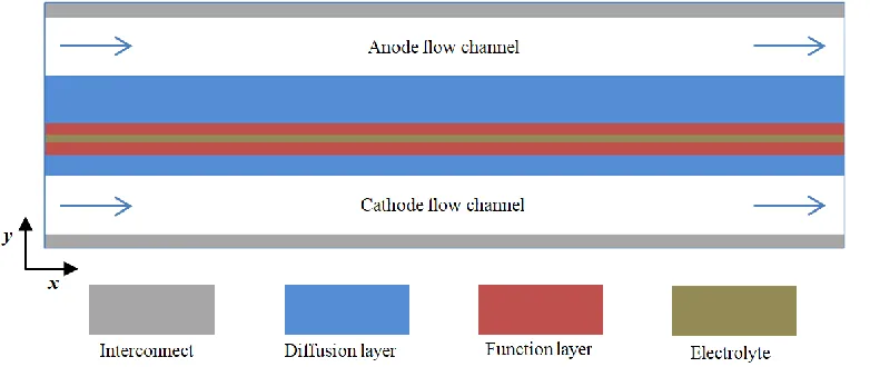
Figure 1. Schematic of anode-supported solid oxide fuel cells.

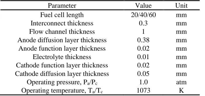
Table 1. SOFC geometric parameters and operating conditions

Parameter Value Unit

Fuel cell length 20/40/60 mm

Interconnect thickness 0.3 mm

Flow channel thickness 1 mm

Anode diffusion layer thickness 0.38 mm Anode function layer thickness 0.02 mm

Electrolyte thickness 0.01 mm

Cathode function layer thickness 0.02 mm Cathode diffusion layer thickness 0.05 mm Operating pressure, Pa/Pc 1.0 atm

Operating temperature, Ta/Tc 1073 K

The assumptions used in this study are as follows: steady state; laminar flow; incompressible gas; isotropic and homogeneous electrodes; neglected radiation heat transfer. The mass equation, momentum equation, species equation, energy equation and charge equation are solved to describe the transport processes in SOFCs. And the governing equations are connected and coupled with each other through the source/sink terms.

2.2 Governing equations

Mass conservation equation:

∇ ⋅ (𝜌𝑢⃗ ) = 𝑆𝑚𝑎𝑠𝑠 (1)

where ρ and 𝑢⃗ are the mixture fluid density and velocity, respectively. Smass is determined by

the mass consumption or generation caused by the electrochemical reaction.

𝑆_{𝑚𝑎𝑠𝑠} = 𝑆_𝐻2 + 𝑆_𝐻2𝑂(Anode) (2)

𝑆_{𝑚𝑎𝑠𝑠} = 𝑆_𝑂2(Cathode) (3)

Momentum conservation equation:

∇ ⋅ (𝜌𝑢⃗ 𝑢⃗ ) = ∇ ∙ (𝜇∇𝑢⃗ ) − ∇𝑃 + 𝑆𝑚𝑜𝑚 (4)

where P is the pressure and μ is the dynamic viscosity. Smom is the source term of momentum

equation. In the porous regions, the Darcy’s law is employed.

𝑆_𝑚𝑜𝑚 = −𝜇

𝐾𝑢⃗ (5)

where K is the permeability. Species conservation equation:

∇ ⋅ (𝜌𝑢⃗ 𝑌_𝑖) = ∇ ∙ (𝜌𝐷𝑒𝑓𝑓,𝑖∇𝑌𝑖) + 𝑆𝑖 (6)

where Yi is the mass fraction and Deff,iis the effective diffusivity. Si is the consumption or

generation amount of the ith (H2, O2, H2O) species.

𝑆𝐻2 = −

𝑗𝑎

2𝐹𝑀𝐻2 (7)

𝑆𝑂2 = −

𝑗𝑐

4𝐹𝑀𝑂2 (8)

𝑆𝐻2𝑂 =

𝑗𝑎

Energy conservation equation:

∇ ⋅ (𝜌𝑐_𝑝𝑢⃗ 𝑇) = ∇ ∙ (𝑘_𝑒𝑓𝑓∇T) + 𝑆_𝑇 (10)

where cp is the specific heat and keff is the effective thermal conductivity. The irreversible,

reversible and ohmic heat generation terms are included in the source term of energy equation.

𝑆_𝑇 = 𝑗_𝑎,𝑐|𝜂_𝑎,𝑐| + 𝑗_𝑎,𝑐𝑇Δ𝑆

𝑛𝐹 + 𝜎𝑒𝑓𝑓,𝑖‖∇ϕ𝑖‖

2_{+ 𝜎}

𝑒𝑓𝑓,𝑠‖∇ϕ𝑠‖2 (11)

Charge conservation equation:

∇ ⋅ (𝜎_{𝑒𝑓𝑓,𝑒}∇𝜙_𝑒) + 𝑆_𝑒 = 0 (12)

∇ ⋅ (𝜎𝑒𝑓𝑓,𝑖∇𝜙𝑖) + 𝑆𝑖 = 0 (13) where σeff,e is the effective electronic conductivity, σeff,i is the effective ionic conductivity.

𝑆𝑒 = −𝑗𝑎 𝑆𝑖 = +𝑗𝑎 (Anode) (14)

𝑆_𝑒 = +𝑗_𝑐 𝑆_𝑖 = −𝑗_𝑐 (Cathode) (15)

The corresponding expressions and parameters related to the mathematical model are summarized in Tables 2 and 3, respectively. In addition, more detailed information about the model can be found in [16].

2.3 Numerical implementation and boundary conditions

The commercial software ANSYS FLUENT is used for the implementation of the present mathematical model. At the inlet of anode and cathode flow channels, the velocity, temperature, and species mass fractions are prescribed. At the outlet of anode and cathode flow channels, a pressure-outlet boundary condition is assigned. Constant electric potentials (ϕe=0 and ϕe=Vcell) are specified at

the anode and cathode terminal walls, respectively. And the adiabatic boundary condition is specified at all the surrounding walls. Detailed boundary conditions are summarized in Table 4.

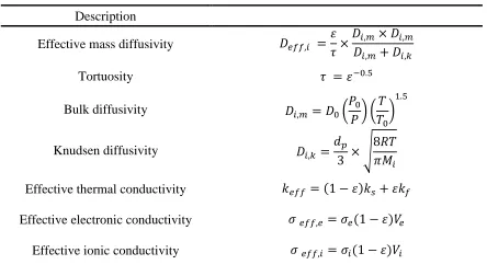
Table 2. Complementary expressions

Description

Effective mass diffusivity 𝐷𝑒𝑓𝑓,𝑖 =

𝜀 𝜏×

𝐷_𝑖,𝑚× 𝐷_𝑖,𝑚 𝐷_𝑖,𝑚+ 𝐷_𝑖,𝑘

Tortuosity 𝜏 = 𝜀−0.5

Bulk diffusivity _{𝐷𝑖,𝑚 = 𝐷0(}𝑃0

𝑃) ( 𝑇 𝑇0

)

1.5

Knudsen diffusivity 𝐷𝑖,𝑘 =

𝑑_𝑝 3 × √

8𝑅𝑇 𝜋𝑀𝑖

Effective thermal conductivity 𝑘𝑒𝑓𝑓 = (1 − 𝜀)𝑘𝑠+ 𝜀𝑘𝑓 Effective electronic conductivity 𝜎 _{𝑒𝑓𝑓,𝑒} = 𝜎_𝑒(1 − 𝜀)𝑉_𝑒

Anode electronic conductivity _{𝜎𝑎,𝑒 =}9.5 × 10 7

𝑇 𝑒𝑥𝑝(− 1150

𝑇 )

Cathode electronic conductivity _{𝜎𝑐,𝑒 =} 4.2 × 10 7

𝑇 𝑒𝑥𝑝(− 1200

𝑇 )

Ionic conductivity 𝜎_𝑖 = 3.34 × 104_{𝑒𝑥𝑝(−}10300

𝑇 )

Anode volumetric current density 𝑗𝑎 = 𝑖𝑎 𝑟𝑒𝑓

𝑎𝑒𝑓𝑓(

𝐶𝐻2

𝐶_𝐻𝑟𝑒𝑓₂ )

𝛾𝑎

[𝑒𝛼𝑎𝐹𝜂𝑎/𝑅𝑇_{− 𝑒}−𝛼𝑐𝐹𝜂𝑎/𝑅𝑇_]

Cathode volumetric current density 𝑗𝑐 = 𝑖𝑐𝑟𝑒𝑓𝑎𝑒𝑓𝑓(

𝐶𝑂2

𝐶_𝑂

2

𝑟𝑒𝑓 ) 𝛾𝑐

[−𝑒𝛼𝑎𝐹𝜂𝑐⁄𝑅𝑇_{+ 𝑒}−𝛼𝑐𝐹𝜂𝑐/𝑅𝑇_]

Anode over-potential 𝜂_𝑎 = ϕ_𝑒− ϕ_𝑖

Cathode over-potential 𝜂_𝑐 = ϕ_𝑒− ϕ_𝑖 − 𝑈_𝑜

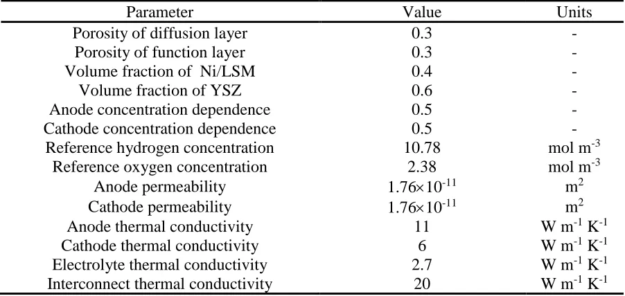
Table 3. Parameters used in the mathematical model

Parameter Value Units

Porosity of diffusion layer 0.3 -

Porosity of function layer 0.3 -

Volume fraction of Ni/LSM 0.4 -

Volume fraction of YSZ 0.6 -

Anode concentration dependence 0.5 -

Cathode concentration dependence 0.5 -

Reference hydrogen concentration 10.78 mol m-3

Reference oxygen concentration 2.38 mol m-3

Anode permeability 1.7610-11 _m2

Cathode permeability 1.7610-11 m2

Anode thermal conductivity 11 W m-1 K-1

Cathode thermal conductivity 6 W m-1 K-1

Electrolyte thermal conductivity 2.7 W m-1 K-1

Interconnect thermal conductivity 20 W m-1 _K-1

Table 4. Boundary conditions

Description Conditions Value Units

Top wall Electrical potential 0 V

Bottom wall Electrical potential 0.7 V

Velocity 0.3 m/s

Fuel inlet Mass fraction H2:H2O=0.95:0.05 -

Temperature 1073 K

Velocity 3 m/s

Air inlet Mass fraction O2:N2=0.233:0.767 -

Temperature 1073 K

Fuel outlet Pressure 0 Pa

3. RESULTS AND DISCUSSION

Figure 2. Comparison between the numerical results and experimental data.

Prior to numerical simulations, a model validation is carried out. As shown in Fig. 2, it is clearly seen that the numerical results show good agreement with the experimental data reported in [17]. For the model validation, the geometric parameters and operating parameters reported in the experiment are adopted. The experimental operating temperature is 1073 K, and the operating pressure is 1.0 atm. Air and humidified hydrogen were introduced into the cathode and anode sides with the flow rate of 500 sccm and 200 sccm, respectively.

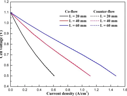
Figure 3. Cell performance of SOFCs with different cell lengths.

are 0.35 A/cm2_{, 0.69 A/cm}2 _{and 1.0 A/cm}2_{, respectively. At the cell voltage 0.5 V, the corresponding}

current densities of three cases are 0.61 A/cm2, 1.11 A/cm2 and 1.47 A/cm2, respectively. The reaction zone is gradually increased when the cell length is increased from 20 mm to 60 mm. This means that the consumption amount of hydrogen and oxygen is increased. Accordingly, the generated electricity is also increased.

Figure 4. Hydrogen mass fraction distributions at the anode diffusion layer and function layer interface of SOFCs with different cell lengths: (a) co-flow arrangement (b) counter-flow arrangement.

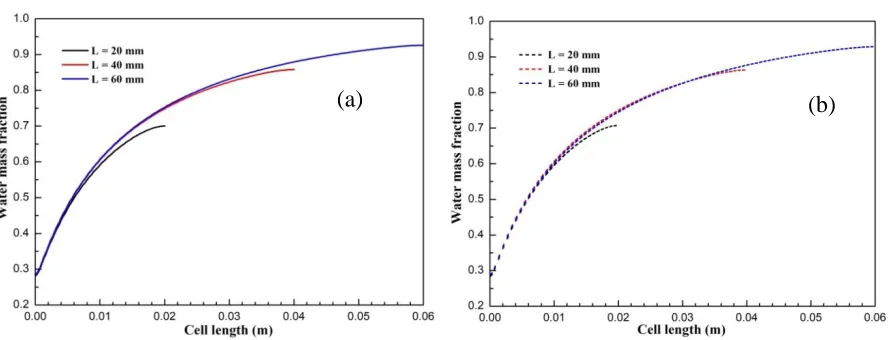
Figure 5. Water mass fraction distributions at the anode diffusion layer and function layer interface of SOFCs with different cell lengths: (a) co-flow arrangement (b) counter-flow arrangement.

(a)

(a) _(b)

Figure 6. Oxygen mass fraction distributions at the cathode diffusion layer and function layer interface of SOFCs with different cell lengths: (a) co-flow arrangement (b) counter-flow arrangement.

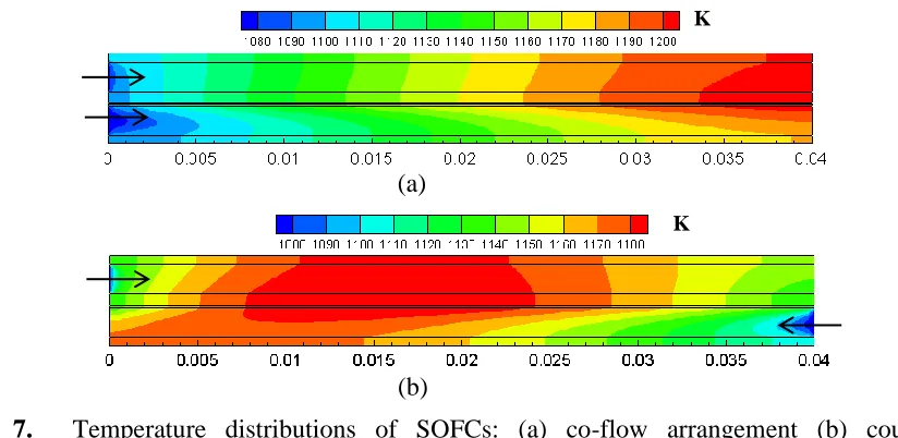
Figure 7. Temperature distributions of SOFCs: (a) co-flow arrangement (b) counter-flow arrangement.

The mass fraction of hydrogen distributions along the cell length direction at cell voltage 0.7 V are shown in Figures 4. It is shown that hydrogen mass fraction is gradually decreased along the cell length direction. This is because hydrogen is consumed and water is simultaneously produced due to the electrochemical reactions occurring in the function layers. For the co-flow arrangement, hydrogen mass fraction of three cases is decreased from 0.719 to 0.3, from 0.716 to 0.142 and from 0.715 to 0.074, respectively. For the counter-flow arrangement, hydrogen mass fraction of three cases is decreased from 0.717 to 0.292, from 0.712 to 0.136 and from 0.712 to 0.071, respectively. The mass fraction of water distributions along the cell length direction at cell voltage 0.7 V are shown in Figures 5. It is shown that water mass fraction is gradually increased along the cell length direction. For the co-flow arrangement, water mass fraction of three cases is increased from 0.281 to 0.7, from 0.284 to 0.858 and from 0.285 to 0.926, respectively. For the counter-flow arrangement, water mass fraction of three cases is increased from 0.283 to 0.707, from 0.287 to 0.863 and from 0.287 to 0.929, respectively. In addition, oxygen mass fraction distributions along the cell length direction at cell

K

(b)

K

(a)

voltage 0.7 V are presented in Figure 6. The mass fraction is gradually decreased due to the consumption of oxygen caused by the electrochemical reactions. It is also observed that the slope of mass fraction profile is not changed by the cell length variation. For the co-flow arrangement, oxygen mass fraction of three cases is decreased from 0.23 to 0.219, from 0.23 to 0.21 and from 0.23 to 0.202, respectively. For the counter-flow arrangement, oxygen mass fraction of three cases is decreased from 0.23 to 0.219, from 0.23 to 0.21 and from 0.23 to 0.202, respectively. Similar mass fraction distributions of hydrogen, water vapor and oxygen can be found in [13-14,18].

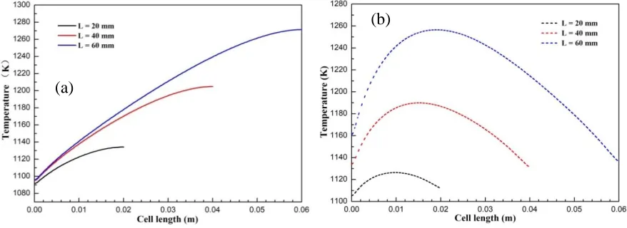
Figure 8. Temperature distributions at the anode diffusion layer and function layer interface of SOFCs with different cell lengths: (a) co-flow arrangement (b) counter-flow arrangement. The temperature distributions at cell voltage 0.7 V are shown in Figure 7. For the co-flow arrangement case, the minimum temperature appears at the cell inlet region and the maximum temperature occurs at the cell outlet region. For the counter-flow arrangement case, the minimum temperature appears at the cell inlet region and the maximum temperature occurs at regions close to fuel side. Similar temperature distributions of SOFCs with co-flow and counter-flow arrangements can also be found in [14, 16, 19-20]. In addition, the local temperature distributions at the anode diffusion layer and function layer interface are shown in Figure 8. For the co-flow arrangement, the temperature of three cases is increased from 1091.4 K to 1134.3 K, from 1094.9 K to 1204.8 K, and from 1095.7 K to 1271.4 K, respectively. For the counter-flow arrangement, the maximum temperature of three cases is 1126.4 K, 1189.9 K and 1256.5 K, respectively.

4. CONCLUSIONS

In this study, a two-dimensional mathematical model is developed and applied to study the transport phenomena in anode-supported SOFCs. The mass, momentum, species, temperature and charge conservation equations are solved, and the effect of cell length on performance and transport phenomena of SOFCs is analyzed and discussed.

(a)

The cell performance is significantly improved with increasing cell length. And the cell performance of SOFCs with a fixed cell length is not changed by the flow arrangement. For the co-flow arrangement, the temperature is gradually increased along the co-flow direction. For the counter-flow arrangement, the temperature is gradually increased to a maximum temperature, and then gradually decreased along the flow direction. The local distributions of hydrogen, oxygen and water are also affected by the cell length and flow arrangement. The present study provides detailed information on the transport phenomena of SOFCs with different cell lengths and flow arrangements.

ACKNOWLEDGMENTS

The authors acknowledge the financial supports from National Natural Science Foundation of China (No.51606013, No.51779025 and No.21676040). This work is also supported by the Fundamental Research Funds for the Central Universities of China (No.3132019191 and No.3132019187).

Nomenclature

a effective surface area, m-1 c mole concentration, mol m-3 cp specific heat, J kg-1 K-1

d diameter, m D diffusivity, m2 _s-1

F Faraday constant, 96485 C mol-1 j volumetric current density, A m-3 k thermal conductivity, W m-1 _K-1

K permeability, m2

M molecular weight, kg mol-1 P pressure, Pa

R universal gas constant, 8.314 J mol-1 K-1 S source term

T temperature, K

𝑢⃗ velocity vector, m/s

U thermodynamic equilibrium potential, V V voltage, V

Y mass fraction Greek Symbols

α transfer coefficient γ concentration dependence ε Porosity

η over-potential, V μ dynamic viscosity, Pa s ρ density, kg m-3

σ electronic/ionic conductivity, S m-1 τ Tortuosity

Superscripts and Subscripts

a Anode

c cathode

e electron

eff effective

f fluid

g gas

i ith species/ion mass mass equation mom momentum equation

p pore

ref reference

s solid

T temperature equation

References

1. S. Mekhilef, R. Saidur, and A. Safari, Renew. Sust. Energ. Rev.,16 (2012) 981. 2. P. Aguiar, C.S. Adjiman, and N.P. Brandon, J. Power Sources, 138 (2004) 120.

3. V. Menon, A. Banerjee, J. Dailly, and O. Deutschmann, Appl. Energy, 149 (2015) 161. 4. J. Kupecki, K. Motylinski, and J. Milewski, Appl. Energy, 227 (2018) 198.

5. M.M. Hussain, X. Li, and I. Dincer, J. Power Sources, 161 (2006) 1012. 6. M. Ni, M.K.H. Leung, and D.Y.C. Leung, J. Power Sources, 168 (2007) 369.

7. S. Su, X. Gao, Q. Zhang, W. Kong, and D. Chen, Int. J. Electrochem. Sci., 10 (2015) 2487.

8. S.Q. Yang, T. Chen, Y. Wang, Z.B. Peng, and W.G. Wang, Int. J. Electrochem. Sci., 8 (2013) 2330. 9. M. Andersson, J. Yuan, and B. Sunden, Fuel Cells, 14 (2014) 177.

10. V.A. Danilov, and M.O. Tade, Int. J. Hydrogen Energy, 34 (2009) 8998. 11. M. Canavar, and B. Timurkutluk, J. Power Sources, 346 (2017) 49.

12. M. Saied, K. Ahmed, M. Nemat-Alla, M. Ahmed, and M. Ei-Sebaie, Int. J. Hydrogen Energy, 43 (2018) 20931.

13. I. Khazaee, and A. Rava, Energy, 119 (2017) 235.

14. Q.W. Shen, L.N. Sun, and B.W. Wang, Int. J. Electrochem. Sci., 14 (2019) 1698.

15. H. Mahcene, H.B. Moussa, H. Bouguettaia, D. Bechki, S. Babay, and M.S. Meftah, Int. J. Hydrogen Energy, 36 (2011) 4244.

16. J.M. Park, D.Y. Kim, J.D. Baek, Y. Yoon, P. Su, and S. Lee, Energies, 11 (2018) 473.

17. Z.G. Zhang, D.T. Yue, C.R. He, S. Ye, W.G. Wang, and J.L. Yuan, Heat Mass Transf., 50 (2014) 1575.

18. H. Mahcene, H.B. Moussa, H. Bouguettaia, D. Bechki, S. Babay and M.S. Meftah, Int. J. Hydrogen Energy, 36 (2011) 4244.

19. A. Yahya, R. Rabhi, H. Dhahri and K. Slimi, Powder Technol., 338 (2018) 402.

20. Z. Zhang, J. Chen, D. Yue, G. Yang, S. Ye, C. He, W. Wang, J. Yuan and N. Huang, Energies, 7 (2014) 80.