This is a repository copy of Setar Modelling of Traffic Count Data.. White Rose Research Online URL for this paper:
http://eprints.whiterose.ac.uk/2186/
Monograph:
Watson, S.M., Clark, S.D., Redfern, E. et al. (1 more author) (1992) Setar Modelling of Traffic Count Data. Working Paper. Institute of Transport Studies, University of Leeds , Leeds, UK.
Working Paper 387
eprints@whiterose.ac.uk https://eprints.whiterose.ac.uk/ Reuse
See Attached
Takedown
If you consider content in White Rose Research Online to be in breach of UK law, please notify us by
White Rose Research Online
http://eprints.whiterose.ac.uk/Institute of Transport Studies
University of Leeds
This is an ITS Working Paper produced and published by the University of Leeds. ITS Working Papers are intended to provide information and encourage discussion on a topic in advance of formal publication. They represent only the views of the authors, and do not necessarily reflect the views or approval of the sponsors.
White Rose Repository URL for this paper: http://eprints.whiterose.ac.uk/2186/
Published paper
Watson, S.M., Clark, S.D., Redfern, E., Tight, M.R. (1992) Setar Modelling of Traffic Count Data. Institute of Transport Studies, University of Leeds. Working Paper 387
UNIVERSITY OF LEEDS
Institute for Transport Studies
ITS Working Paper 387
ISSN 0142-8942September 1992
SETAR MODELLING OF TRAFFIC COUNT DATA
SM Watson
SD Clark
E Redfern
(Department of Statistics)MR Tight
This work was undertaken on a project sponsored by the Science and Engineering Research Council (Grant Ref:)
Project title: .
ITS Working Papers are intended to provide information and encourage discussion on a topic in advance of formal publication. They represent only the views of the authors, and do not
CONTENTS
Page
1.INTRODUCTION 1
2.MODEL FORM 2
3.DATA DESCRIPTION 2
4.SETAR MODELLING RESULTS 3
5.CONCLUSIONS 4
SETAR MODELLING OF TRAFFIC COUNT DATA
1.INTRODUCTION
As part of a SERC funded project investigating outlier detection and replacement with transport data, univariate Box-Jenkins (1976) models have already been successfully applied to traffic count series (see Redfern et al, 1992). However, the underlying assumption of normality for ARIMA models implies they are not ideally suited for time series exhibiting certain behavioural characteristics. The limitations of ARIMA models are discussed in some detail by Tong (1983), including problems with time irreversibility, non-normality, cyclicity and asymmetry. Data with irregularly spaced extreme values are unlikely to be modelled well by ARIMA models, which are better suited to data where the probability of a very high value is small. Tong (1983) argues that one way of modelling such non-normal behaviour might be to retain the general ARIMA framework and allow the white noise element to be non-gaussian. As an alternative he proposes abandoning the linearity assumption and defines a group of non linear structures, one of which is the Self-Exciting Threshold Autoregressive (SETAR) model. The model form is described in more detail below but basically consists of two (or more) piecewise linear models, with the time series "tripping" between each model according to its value with respect to a threshold point. The model is called "Self-Exciting" because the indicator variable determining the appropriate linear model for each piece of data is itself a function of the data series. Intuitively this means the mechanism driving the alternation between each model form is not an external input such as a related time series (other models can be defined where this exists), but is actually contained within the series itself. The series is thus Self-Exciting.
The three concepts embedded within the SETAR model structure are those of the threshold, limit cycle and time delay, each of which can be illustrated by the diverse applications such models can take.
The threshold can be defined as some point beyond which, if the data falls, the series structure changes inherently and so an alternative linear model form would be appropriate. In hydrology this is seen as the non-linearity of soil infiltration, where at the soil saturation point (threshold) a new model for infiltration would become appropriate.
Limit cycles describe the stable cyclical phenomena which we sometimes observe within time series. The cyclical behaviour is stationary, ie consists of regular, sustained oscillations and is an intrinsic property of the data. The limit cycle phenomena is physically observable in the field of radio-engineering where a triode valve is used to generate oscillations (see Tong, 1983 for a full description). Essentially the triode value produces self-sustaining oscillations between emitting and collecting electrons, according to the voltage value of a grid placed between the anode and cathode (thereby acting as the threshold indicator).
The third essential concept within the SETAR structure is that of the time delay and is perhaps intuitively the easiest to grasp. It can be seen within the field of population biology where many types of non-linear model may apply. For example within the cyclical oscillations of blowfly population data there is an inbuilt "feedback" mechanism given by the hatching period for eggs, which would give rise to a time delay parameter within the model. For some processes this inherent delay may be so small as to be virtually instantaneous and so the delay parameter could be omitted.
2
Canadian Lynx trapping series and for modelling riverflow systems (Tong, Thanoon & Gudmundsson, 1984). Here we investigate their applicability with time series traffic counts, some of which have exhibited the type of non-linear and cyclical characteristics which could undermine a straightforward linear modelling process.
2.MODEL FORM
A general form for the Single Threshold SETAR (k) model is given by
Yt + 1(1) Yt-1 + . . . + k(1) Yt-k = µ1 + t if yt-d≤ C ⎫
⎬ . . . (1) yt + 1(2) Yt-1 + . . . + k(2) Yt-k = µ2 + t if yt-d > C ⎭
where d is integer ≥ 1 ("delay" parameter)
k is integer ≥ 0 (Threshold Autoregressive order)
i(1), i(2) are real coefficients, i(1) applying to region 1 and i(2) to region 2.
C is a single threshold value.
Hence, for a single threshold with parameter C, there exist two piecewise linear models with the data separated into each of two regions according to a previous value with respect to the threshold.
Here we use an algorithm by Petruccelli and Davies (1985) to fit a Threshold model up to order TAR(3) ie with a maximum of 3 autoregressive parameters. The algorithm identifies and estimates TAR models using Akaiki's (1977) AIC criterion with a potential maximum of 4 Thresholds. This corresponds to a maximum of 5 regions within the data. A portmanteau test is used to detect non-linearity in the series and the AIC value used to locate the threshold.
When SETAR models were applied to machined surface profiles (see Spedding, 1983 and Watson, 1987) a single threshold was located with two distinct regions in the data. Observations contained wholly within the first region were found to be deep scratches in the machined surface and could therefore be thought of as "outliers" within the series. It is conjectured that a similar phenomena could arise with time series transport data, with missing or outlying data being separated into a distinct region.
3.DATA DESCRIPTION
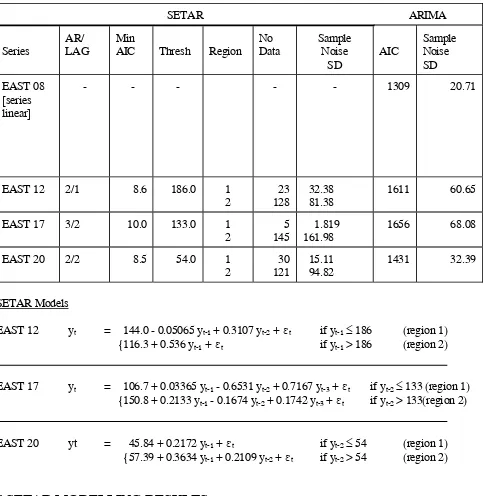
Table 1: SETAR and ARIMA fits to T/B East Series
SETAR ARIMA
Series
AR/ LAG
Min
AIC Thresh Region No Data Sample Noise SD AIC Sample Noise SD EAST 08 [series linear]
- - - - - 1309 20.71
EAST 12 2/1 8.6 186.0 1 2
23 128
32.38 81.38
1611 60.65
EAST 17 3/2 10.0 133.0 1 2
5 145
1.819 161.98
1656 68.08
EAST 20 2/2 8.5 54.0 1 2
30 121
15.11 94.82
1431 32.39
SETAR Models
EAST 12 yt = 144.0 - 0.05065 yt-1 + 0.3107 yt-2 + t if yt-1≤ 186 (region 1)
{116.3 + 0.536 yt-1 + t if yt-1 > 186 (region 2)
EAST 17 yt = 106.7 + 0.03365 yt-1 - 0.6531 yt-2 + 0.7167 yt-3 + t if yt-2≤ 133 (region 1)
{150.8 + 0.2133 yt-1 - 0.1674 yt-2 + 0.1742 yt-3 + t if yt-2 > 133(region 2)
EAST 20 yt = 45.84 + 0.2172 yt-1 + t if yt-2≤ 54 (region 1)
{57.39 + 0.3634 yt-1 + 0.2109 yt-2 + t if yt-2 > 54 (region 2)
4.SETAR MODELLING RESULTS
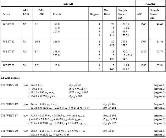
A comprehensive summary of modelling results obtained using the algorithm of Petruccelli and Davies (1985) is given within Tables 1 and 2, together with some diagnostics from ARIMA fits. In each table the value of the threshold parameter C is shown, and it can be seen from Table 2 that for westbound traffic at 08:00 a total of 3 thresholds (giving 4 regions) were needed. The total number of observations falling within each region are also indicated, and for some (eg region 1, T/B East 17:00) this is quite a small number. The expanded model form and region definitions are shown below Tables 1 and 2.
4
From Table 1, series T/B East 08:00 was determined to be linear according to the portmanteau criteria and so a SETAR structure was not applied. The remaining three Eastbound series were found to be non-linear with a single threshold. In each case a small proportion of the data was contained in the first region and the sample noise standard deviation for that region was quite small. For the second region (containing the bulk of the data), a much larger standard deviation was recorded for the noise. The full model form is shown at the bottom of Table 1. Relatively few parameters were needed in each case, with the maximum order being a TAR (3) for T/B East 17:00. However, it should be noted that this was the highest order permitted within the algorithm. Although it is difficult to draw a direct comparison, the AIC and sample noise SD resulting from univariate fits are indicated in columns 8 and 9. Clearly the non-linear fit has produced a substantially lower AIC value and whilst the noise standard deviation is also much reduced for region 1, this is not the case for region 2 containing most of the observations.
The delay parameter d was selected as d=1 for T/B East 12:00 and d=2 for T/B East 17:00 and T/B East 20:00, representing a small inherent delay within the process. It is conjectured that without programming restrictions a value of d=7 may have evolved in order to reflect the known 7 day periodicity of the data. Further substantial programming modifications would be required to overcome the existing restriction 1 < d < k < 3.
A slightly more complex situation arises with the Westbound data (Table 2), where all four series were found to be non-linear and two series contained more than one threshold. With the exception of T/B West 08:00 a TAR(3) was needed in each case. Although a low order model suffices for T/B West 08:00 it is modelled using 3 thresholds.
Considering the position of observations with regard to thresholds, a differing picture emerges for the 3 non-linear East bound series than that for West bound flows. Thresholds have been marked on the series plots (Figures 2 to 8) for reference. The single threshold determined for East bound traffic places those observations with the lowest values (including missing values coded as zero) into one region. Whilst these may or may not be genuine outliers, high extreme values, such as those observed visually in T/B East 20:00 have not been separated out.
A similar case exists for T/B West 12:00 and T/B West 20:00, with only the lowest 7 data points in region 1 for the latter. For T/B West 08:00 and T/B West 17:00, whilst a small collection of observations have been placed in region 1, an even smaller number are separated into region 2. Interpretationally this is less clear, but it seems those data in region 2 may be the lowest dips in the cyclical lows of the series.
Table 2:SETAR and ARIMA fits the T/B WEST Series
SETAR ARIMA
Series
AR/ LAG
Min
AIC Thresh Region
No Data Sample Noise SD AIC Sample Noise SD
WEST 08 1/1 8.3 72.0
77.0 107.0 1 2 3 4 22 5 11 114 36.77 7.08 43.9 70.76
1543 46.40
WEST 12 3/1 10.1 166.0 1
2
22 128
105.8 159.2
1705 81.46
WEST 17 3/2 8.7 198.0
225.0 1 2 3 18 5 127 30.2 0.4014 94.9
1580 52.74
WEST 20 3/1 8.7 63.0 1
2
7 143
6.99 80.62
1385 27.86
SETAR Models
T/B WEST 08 yt = 145.3 + t if yt-1≤ 72 (region 1)
{ 56.2 + t if 72 < yt-1≤ 77 (region 2)
{ 482.2 - 3.93 yt-1 + t if 77 < yt-1≤ 107 (region 3)
{ 114.8 + 0.258 yt-1 + t if yt-1 > 107 (region 4)
T/B WEST 12 yt = 341.6 - 1.107 yt-1 + t if yt-1≤ 166 (region 1)
{ 111.6 + 0.4851 yt-1 - 0.01547 yt-2 + 0.1916 yt-3 + t if yt-1 > 166 (region 2)
T/B WEST 17 yt = 315.3 - 0.1539 yt-1 - 0.3865 yt-2 + 0.1686 yt-3+ t if yt-2≤ 198 (region 1)
{ -48.45 - 0.9842 yt-1 + 0.428 yt-2 - 9.44 yt-3+ t if yt-2≤ 225 (region 2)
{ 233.6 + 0.2288 yt-1 - 0.2543 yt-2 + 0.2619 yt-3+ t if yt-2 > 225 (region 3)
T/B WEST 20 yt = 158.3 - 1.187 yt-1 + -0.1063yt-2 - 0.3379yt-3 + t if yt-1≤ 63 (region 1)
{102.1 + 0.2852 yt-1 + tif yt-1 < 63 (region 2)
5.CONCLUSIONS
Results presented here refer to only preliminary findings from a limited number of traffic count time series. However the degree of success indicated by low AIC and simpler model forms indicates a wider study of the applicability of SETAR structures may be warranted. Certainly the underlying non-linearity primarily illustrated through non-stationary and cyclical behaviour has been confirmed. Further programming work could allow the inherent 7-day periodicity to be incorporated and it would be of interest to observe the SETAR Model fits if the missing values were replaced. It is not clear at this stage why high extreme values have not been detected and it could be a worthy exercise to `invert' the series and re-model.
6
6.REFERENCES
BOX, G E P and JENKINS, G M (1976). Time series analysis, forecasting and control. Holden-Day.
PETRUCCELLI, J D and DAVIES, N (1985). A portmanteau test for sector-type non-linear time series. Research Report MSOR/9/85, Trent Polytechnic, Nottingham.
PRIESTLY, M B (1980) State dependent models: a general approach to non-linear time series analysis. JTSA Volume 1, 47-71.
PRIESTLY, M B (1981) Spectral analysis and time series. Volume 2. Multivariate Series, Production and Control.
REDFERN, E J, CLARK, S D, WATSON, S M and TIGHT, M R (1992). Application of Univariate Box-Jenkins models to time series traffic data. ITS Working Paper Institute for Transport Studies, University of Leeds, Leeds.
SPEDDING, T A (1983). The machined surface - statistics and characterisation. PhD Thesis, Coventry (Lanchester) Polytechnic.
TONG, H and LIM, K S (1980). Threshold autoregression, limit cycles and cyclical data. JRSS (B), Volume 42, 245-292.
TONG H, THANOON, B and GUDMUNDSSON, G (1984). Threshold time series modelling of two Icelandic Riverflow Systems. Technical Report No 17, Dept Statistics, Chinese University of Hong Kong.
WATSON, S M (1987). Non-normality in time series analysis. PhD Thesis, Trent Polytechnic, Nottingham.
7
g\...\wptnlist\wp387.smw