This is a repository copy of
Freeway traffic estimation within particle filtering framework
.
White Rose Research Online URL for this paper:
http://eprints.whiterose.ac.uk/82258/
Version: Submitted Version
Article:
Mihaylova, L., Boel, R. and Hegyi, A. (2007) Freeway traffic estimation within particle
filtering framework. Automatica, 43 (2). 290 - 300. ISSN 0005-1098
https://doi.org/10.1016/j.automatica.2006.08.023
[email protected] https://eprints.whiterose.ac.uk/ Reuse
Unless indicated otherwise, fulltext items are protected by copyright with all rights reserved. The copyright exception in section 29 of the Copyright, Designs and Patents Act 1988 allows the making of a single copy solely for the purpose of non-commercial research or private study within the limits of fair dealing. The publisher or other rights-holder may allow further reproduction and re-use of this version - refer to the White Rose Research Online record for this item. Where records identify the publisher as the copyright holder, users can verify any specific terms of use on the publisher’s website.
Takedown
If you consider content in White Rose Research Online to be in breach of UK law, please notify us by
Brief paper
Freeway Traffic Estimation
Within Particle Filtering Framework
Lyudmila Mihaylova
∗
,a,Ren´
e Boel
b, Andreas Hegyi
caDepartment of Communication Systems, Lancaster University, South Drive, Lancaster LA1 4WA, UK
bUniversity of Ghent, SYSTeMS Research Group, B-9052 Zwijnaarde, Belgium
cDelft University of Technology, Delft Center for Systems and Control, Mekelweg 2, 2628 CD Delft, The Netherlands
Abstract
This paper formulates the problem of real-time estimation of traffic state in freeway networks by means of particle filtering framework. A particle filter (PF) is developed based on a recently proposed speed-extended cell-transmission model of freeway
traffic. The freeway is considered as a network of components representing different freeway stretches called segments. The
evolution of the traffic in a segment is modelled as a dynamic stochastic system, influenced by states of neighbour segments.
Measurements are received only at boundaries between some segments and averaged within possibly irregular time intervals. This limits the measurement update in the PF to only these time instants when a new measurement arrives, with possibly many state updates in between consecutive measurement updates. The PF performance is validated and evaluated using synthetic and real traffic data from a Belgian freeway. An Unscented Kalman filter is also presented. A comparison of the particle filter with the Unscented Kalman filter is performed with respect to accuracy and complexity.
Keywords: Bayesian estimation, particle filtering, macroscopic traffic models, stochastic systems, unscented Kalman filter
1 Motivation
Traffic state estimation and prediction is of paramount importance for on-line road traffic management, effi-ciency and safety. Vehicular traffic is characterised with highly nonlinear behaviour (Helbing, 2002), with many interactions between vehicles, and high complexity which makes this problem challenging. This behaviour can be described bymacroscopicmodels (Hoogendoorn and Bovy, 2001; Kotsialos et al., 2002; Helbing, 2002) that are suitable for real-time problems in view the fact that they represent theaverage traffic behaviour in terms of aggregated variables (flow, density and speed at different locations). Most papers dealing with recur-sive traffic state estimation apply the Extended Kalman filter (EKF) to such macroscopic models. For example (Wang and Papageorgiou, 2005) proposes an EKF to es-timate the unknown parameters and states of a stochas-tic version of the macroscopic freeway traffic flow model METANET (Papageorgiou and Blosseville, 1989) of freeway traffic. These estimators have all the advantages and disadvantages of the EKF technique: presumably computationally cheap, but relying on a linearisation of the state and measurement models which can cause
∗ Corresponding author
Email addresses: [email protected](Lyudmila
Mihaylova),[email protected](Ren´e Boel),
[email protected](Andreas Hegyi).
filter divergence. A powerful and scalable approach has recently been developed, known under different names such asparticle filters(PFs) (Doucet et al., 2001; Ristic et al., 2004; Chen, 2003) andbootstrap method (Gordon et al., 1993). All information about the states of interest can be obtained from the conditional distribution of the state given the past observations and the dynamics of the system. It approximates the posterior density func-tion of the state by an empirical histogram obtained from samples generated by a Monte Carlo simulation. Particle filtering allows to cope with uncertainties and nonlinearities of different kinds, nonGaussian noises and hence is suitable for the traffic estimation problem.
In the present paper we formulate the traffic estimation problem within this Bayesian framework and develop a particle filter for freeway traffic flow estimation. This is an extension and generalisation of the results reported in (Mihaylova and Boel, 2004). The structure of the PF fits well to the compositional traffic networks, and it allows for parallelisation for different segments.
In (Sun et al., 2003) a solution to highway traffic es-timation is proposed by a sequential Monte Carlo al-gorithm, the so-called mixture Kalman filtering. First-order traffic models represent the network, i.e. only the traffic density is modelled, distinguishing between the
free-flow modeandcongestion mode. In contrast to (Sun
Li,k Segment i
Ni,k, vi,k
Ni-1,k, vi-1,k Ni+1,k, vi+1,k
Qi-1,k Qi,k
Sensor measurements in tk ≡ts
1 2 i-1 i i+1 n-1 n
Qkin, vkin Qk out, vk out
n+1
[image:3.595.64.260.75.211.2]z1,s zj,s zm,s
Fig. 1. Freeway segments and measurement points.Qiis the
average number of vehicles crossing the boundary between
segmentsiandi+ 1,Niandviare respectively the average
number of vehicles and speed within segmenti.
by a second-order macroscopic model, and we develop a particle filter that estimates both the traffic density and speed. The traffic is described by the recently developed model (Boel and Mihaylova, 2006) that is an extension to the cell-transmission model (Daganzo, 1994). The free-way network is modelled as a sequence of segments (Fig. 1). Sensors are available only at some boundaries be-tween segments. Technological limitations (such as lim-ited bandwidth of communication channels) force one to average these measurements over regular or irregular time intervals before they are transmitted to the centre where the Bayesian update of the conditional densities is carried out (for all segments concurrently).
We investigate the PF performance with respect to accuracy and complexity and we compare it with an-other method suitable for traffic flow estimation, the Unscented Kalman filter (UKF) (Julier and Uhlmann, 2004; Wan and van der Merwe, 2001). The UKF is a derivative-free estimation method, that has proven to outperform the EKF. The UKF can be viewed as a method to approximate the first two moments of the state: the mean and covariance. Unlike the EKF, the UKF does not require calculation of Jacobians and Hessians. Deterministic sampling approach is used to calculate the mean and covariance, by the so-called sigma points. Compared with the EKF’s first-order accuracy, the estimation accuracy of the UKF is to the third order (Taylor series expansion) for any non-linearity. The EKF requires calculation of derivatives for all traffic segments which for the traffic problem with interconnected components is quite complicated. Moreover, divergence problems are not excluded. The UKF is much easier to implement and more accurate. However, the UKF often encounters the ill-conditioned problem of the covariance matrix in practice (though theoretically it is positive semi-definite). Methods for enhancing the numerical properties of the UKF (e.g. as based on singular-value decomposition) can overcome these numerical instabilities (Chen, 2003).
The added values and innovative aspects of this paper as compared to previous investigations include:
1. A general stochastic macroscopic traffic flow model is presented together with measurement equations, suit-able for a PF real-time estimation and prediction.
2. We demonstrate that PF can be efficiently and eas-ily implemented for large compositional models and sparse measurements, received synchronously or
asyn-chronously at intervals, bigger than the state-update
sample time. The developed approach is general and applicable to freeway networks with different topologies.
3. We compare the PF performance with respect to an UKF. We show that the PF estimates are more accu-rate than those of the UKF, nevertheless the PF is more computationally expensive.
The outline of the paper is as follows. Section 2 presents a stochastic macroscopic traffic model for freeway stretches and a model for real-time traffic measure-ments. Bayesian formulation of the traffic estimation problem is given in Section 3. A PF framework for traffic state estimation is developed in Section 4 which takes advantage of the compositional traffic model. Section 5 describes the UKF for traffic estimation that is com-pared with the developed PF. The PF performance is evaluated in Section 6. Conclusions and future research issues are highlighted in Section 7.
2 Freeway Traffic Flow Model
2.1 Compositional Macroscopic Traffic Model
Traffic states are estimated consecutively at discrete time instantst1, t2, . . . , tk, . . ., possiblyasynchronously, based on all the incoming information up to the current time transmitted by sensors to the filter. The overall state vectorxk= (xT1,k,x2,kT , . . . ,xTn,k)T at timetk con-sists of local state vectors xi,k = (Ni,k, vi,k)T, where
Ni,k, [veh], is the number of vehicles counted in segment
i ∈ I ={1,2, . . . n}, and vi,k, [km/h], is their average speed. The traffic state evolution is described by the system of equations
x1,k+1=f1(Qink , vink ,x1,k,x2,k,η1,k), (1)
xi,k+1=fi(xi−1,k,xi,k,xi+1,k,ηi,k), (2) xn,k+1=fn(xn−1,k,xn,k, Q
out
k , voutk ,ηn,k), (3) where fi is specified by the traffic model, Qink is the number of vehicles entering segment 1 during the inter-val ∆tk =tk+1−tk with average speedvkin,Qoutk is the outflow leaving a ‘fictitious’ segmentn+ 1, with an av-erage speedvout
k . ηk is a disturbance vector, reflecting random fluctuations and the effect of modelling errors in the state evolution. Note thatQink ,vink , andQoutk , voutk are respectively, inflow and outflowboundary variables.
Theyare not traffic states and are not estimated. They
are supplied by the traffic detectors. Hence, a chain of in-terconnected segments is considered, together with their boundary conditions.
In this paper the general state-space description (1)-(3) takes a particular form of the recently developed compositional stochastic macroscopic traffic model (Boel and Mihaylova, 2006). This speed-extended cell-transmission model describes the complex traffic be-haviour withforward andbackward propagation of traf-fic perturbations and is suitable for large networks and for distributed processing. The forward and backward traffic perturbations were characterised by (Daganzo, 1994) through deterministic sending and receiving func-tions where piecewise affine representafunc-tions are used. In (Boel and Mihaylova, 2004; Boel and Mihaylova, 2006) speed-dependent random sending and receiving functions are introduced that represent also the evolu-tion of the average speed in each segment. The model is given in concise form as Algorithm 1.
The sending function Si,k for each segment i, having
lengthLi, is calculated by (4).Si,k represents the vehi-cles that “intend to leave” segmentiwithin ∆tk. The
re-ceiving function Ri,k(6). expresses the maximum
num-ber of vehicles that are allowed to enter segmenti+ 1. In (6) Ni+1,kmax characterises themaximum number of vehi-clesthat can simultaneously be present in segmenti+ 1 in ∆tk. Ni+1,kmax depends on the available space,Li+1time the number of lanesℓi+1,k, in segmenti+ 1,on the av-erage lengthAℓof vehicles, the average speedvi+1,kand the time distance td between two vehicles (in order to allow safe driving).
The evolution ofNi,k+1 is governed by the principle of conservation of vehicles (9). The traffic density ρi,k+1, [veh/km/lane], is given by (10). The anticipated density
ρantic
i,k+1is then obtained as a weighed average between the density of segment iand segmenti+ 1, (11). This cor-responds to the drivers’ tendency usually to look ahead when they change their speed. The average vehicle speed
vi,k+1 is a function of the ‘intermediate’ speedvi,k+1interm, calculated in step 5 of Algorithm 1, and of the equilib-rium speed satisfying a speed-density relationve(ρantic
i,k+1) (Kotsialos et al., 2002).
Design traffic parameters are: the free-flow speedvf ree, the critical densityρcrit(density below which the inter-actions between vehicles will be negligible), the density in jam, ρjam, above which the vehicles do not move, and the minimum vehicle speed vmin, the parameters
α ∈ (0,1], 0 < βI < βII, a threshold density value
ρthreshold. Other details for the model can be found in (Boel and Mihaylova, 2004; Boel and Mihaylova, 2006) where this extended cell-transmission model has been validated both against the well established METANET model (Papageorgiou and Blosseville, 1989; Kotsialos et al., 2002), and over real traffic data.
Algorithm 1. The compositional traffic model.
1.Forward wave: fori= 1,2, . . . , n
Si,k =max
³
Ni,kvi,kL.∆itk +ηSi,k, Ni,k
vmin.∆tk
Li
´
(4)
and set Qi,k=Si,k. (5)
2.Backward wave: fori=n, n−1, . . . ,1
Ri,k =Nimax+1,k−Ni+1,k+Qi+1,k, (6)
whereNimax+1,k= (Li+1ℓi+1,k)/(Aℓ+vi+1,ktd).
if Si,k < Ri,k, Qi,k=Si,k, (7)
else Qi,k=Ri,k, vi,k=Qi,kLi/(Ni,k∆tk), (8)
3. Update the number of vehicles inside segments,
fori= 1,2, . . . , n
Ni,k+1=Ni,k+Qi−1,k−Qi,k, (9)
4. Update the density, fori= 1,2, . . . , n
ρi,k+1=Ni,k+1/(Liℓi,k+1), (10) ρantic
i,k+1=αρi,k+1+ (1−α)ρi+1,k+1. (11)
5. Update of the speed, fori= 1,2, . . . , n
vinterm i,k+1 =
(vi−1,kQi−1,k+vi,k(Ni,k−Qi,k)
Ni,k+1 , forNi,k+16= 0, vf, otherwise,
vintermi,k+1 =max(vintermi,k+1 , vmin),
vi,k+1=βk+1vi,kinterm+1 + (1−βk+1)ve(ρantici,k+1) +ηvi,k+1, where
βk+1= (
βI, if |ρantic
i+1,k+1−ρantici,k+1| ≥ρthreshold,
βII otherwise.
2.2 Measurement Model
Sensors (magnetic loops, video cameras, radar detectors) are located at boundaries between some segments. Usu-ally, measurements are collected at the entrance and at the exit of the considered stretch of the road, at the on-ramps and off-on-ramps, etc.
Let us consider m sensors along the stretch. Traffic states are measured at discrete time instants. The over-all measurement vector zs = (zT1,s,zT2,s, . . . ,zTm,s)T at time ts consists of local measurement vectors
zj,s = (Qj,s, vj,s)T, wherej ∈ J = {1,2, . . . , m}.Qj,s is the noisy measurement of the number of vehicles crossing the boundaries between the corresponding segment i and segment i+ 1 during the time interval ∆ts = ts+1−ts, andvj,s is the measured mean speed of these vehicles. The intervals ∆tsare typically several times longer than the intervals ∆tk betweenq succes-sive state update steps, i.e. ∆ts = q∆tk. Given the measurement equation
zs=h(xs,ξs), (12)
framework. We consider the following particular form for equation (12)
zj,s=
ï
Qj,s ¯
vj,s !
+ξj,s, (13)
where ¯Qj,s is the sum of the number of vehicles (cal-culated by the state model) crossing the boundary between segments i and i+ 1 within the interval ∆ts, and ¯vj,sis their average speed. Although Gaussian dis-tributions of the noise vector ξj,s = (ξQj,s, ξvj,s)
T in
(13) has been used previously in the literature (Wang and Papageorgiou, 2005), we propose a more realistic noise model. This is another advantage of the PF: the knowledge of the noise distributions can be utilised for a better state tracking. Based on statistical analysis of different sets of traffic data we found that there are two kinds of measurement errors in the counted vehicles by the video cameras: errors due to false detections,
ξQf alse
j ,s, and errors due to missed vehicles, ξQ missed j ,s. Hence, the measurement error in the observation equa-tion (12) resp. (13) is of the form
ξj,s=Qerrj,s =Q f alse j,s −Q
missed
j,s , (14)
where the number of the vehicles that a detectorjmissed is denoted by Qmissed
j,s , and the number of the false de-tections byQf alsej,s . Analysis of data from video cameras has shown that Qf alsej,s and Qmissedj,s can both be con-sidered independent Poisson random variables with pa-rametersλ1andλ2. Based on our analysis we estimate
λ1+λ2= 2,λ1= 4/3,λ2= 2/3. Then the PDF of the measurement noiseξQi,sis a convolution of the form
p(Qerr
j,s =νi,serr) =
∞
X
νmissed i,s =0
λ(ν
err
i,s+νmissedi,s )
1 e
−λ1
(νerr
i,s +νi,smissed)!
.λ
νmissed i,s
2 e
−λ2
νmissed i,s !
. (15)
Eq. (15) represents the PF likelihood function of the observations over the counted number of vehicles. We assume that the speed noisesξvj,s are Gaussian. Under the assumption that the vehicle counts are statistically independent from the speed measurements, the entire likelihoodp(zs|xs) given the statexsis the product of the likelihood of the measured counts with the likelihood of the measured speeds.
3 Bayesian Estimation of Traffic Flows
Bayesian estimation evaluates the posterior probability
density function (PDF)p(xk|Zk) of the state vectorxk
up to time instant tk given a setZk = {z1, ...,zk} of sensor measurements available at time tk. Within the recursive Bayesian framework (Ristic et al., 2004), the
conditional density functionp(xk|Zk
−1
) of the statexk given a set of measurementsZk−1
is recursively updated according to
p(xk|Zk
−1
) = Z
Rnx
p(xk|xk−1)p(xk−1|Z
k−1
)dxk−1, (16)
p(xk|Zk) =
p(zk|xk)p(xk|Zk
−1
)
p(zk|Zk
−1
) , (17)
wherep(zk|Zk
−1
) is a normalising constant. Therefore, the recursive update ofp(xk|Zk) is proportional to
p(xk|Zk)∝p(zk|xk)p(xk|Zk
−1
). (18)
The state prediction step (16) and the measurement up-date step (17) use respectively the conditional density functions p(zk|xk) andp(xk|xk−1) that are defined by the model from Section 2.1.
4 Particle Filtering for Freeway Traffic
Evaluating (16)-(18) is computationally very expensive. The particle filter technique (Gordon et al., 1993; Doucet et al., 2001) provides an approximate solution to (16)-(18) by a discrete-time recursive update of theposterior
PDFp(xk|Zk) of the state given the measurements The particle filter approximatesp(xk|Zk) by the empirical histogram corresponding to a collection ofM particles
(samples) {x(l)k }M
l=1. To each particlel a weightw (l) k is assigned at timetk (the sum of these weights must be normalised to 1). The weight and the value of all parti-cles together define a histogram that approximates the conditional density function of the state vectorxk. After the arrival of a new observation vectorzs, the particle filter updates the weights according to (18). The cloud of particles evolves with time and depending on the ob-servations, so that the particles represent with sufficient accuracy the true PDF of the state (Doucet et al., 2001).
Aresamplingprocedure introduces variety in the
parti-cles, by eliminating the particles with small weights and by replicating particles with larger weights.
The traffic estimation problem has particularities distin-guishing it from other estimation problems:i) the lim-ited amount of available data from traffic detectors. The number of traffic variables to be estimated is much larger than the number of the traffic variables that are directly observed, and this “interpolation” is an essential con-tribution to the freeway traffic estimation task. ii) the state estimates are highly dependent on the inflowQin,
vinand randomQout,vout boundary variables.
The likelihood functionp(zk|xk) is calculated from (13) only when a measurement arrives, using the predicted state values and the known measurement noise density
Algorithm 2. A Particle Filter for Traffic Estimation.
I. Initialisation:k= 0
Forl= 1, . . . , M, generate samples{x(0l)}from the initial distributionp(x0)and
initial weightsw(0l)= 1/M.
End For
II. Fork= 1,2, . . . ,
(1) Prediction step:
Forl= 1, . . . , M, samplex(kl)∼p(xk|x(kl−)1)
according to (4)-(11) for segments between
two boundaries where measurements arrive
End For
(2) Measurement processing step (only for tk≡ts,
on boundaries between the segments where
measurements are available) compute the weights
Forl= 1, . . . , M
ws(l)=ws(l−)1p(zs|x
(l)
s ),
End For
where the likelihoodp(zs|x(sl))
is calculated by the model (13)
from section 2.2.
Forl= 1, . . . , M
Normalise the weights:wˆ(sl)=ws(l)/PMl=1w (l)
s .
End For
(3) Output:xˆs=PMl=1wˆ (l)
s x(sl),
(4) Selection step (resampling) only fortk≡ts:
Multiply/ Suppress samplesx(sl) with high/ low
importance weightswˆ(sl), in order to obtainM
random samples approximately distributed
accor-ding top(x(sl)|Zs), e.g. by residual resampling.
* Forl= 1, . . . , M, setws(l)= ˆw(sl)= 1/M, End For
(5)k←k+ 1and return to step (1).
function p(ξs). The cloud of weighted particles repre-senting the posterior conditional PDF, is used to map integrals to discrete sums:p(xk|Zk) is approximated by
ˆ
p(xk|Zk)≈ M X
l=1 ˜
wk(l)δ(xk−x(l)k ), (19)
where δ is the delta-Dirac function and ˜wk(l) are the normalised weights of the posterior conditional PDF. New weights are calculated putting more weight on particles that are important according to the posterior probability density function (19). The random sam-ples {x(l)k , l = 1,2, . . . , M} are drawn from p(xk|Zk).
It is often impossible to sample from the posterior density function p(xk|Zk). However, this difficulty is circumvented by making use of the importance sam-pling from a known proposal distribution π(xk|Zk). The transition prior is the most popular choice of the proposal distribution (Wan and van der Merwe, 2001):
π(xk|Zk) = p(xk|xk−1), which in our solution to the traffic problem is the traffic state model. Algorithm 2 presents the PF developed in this paper.
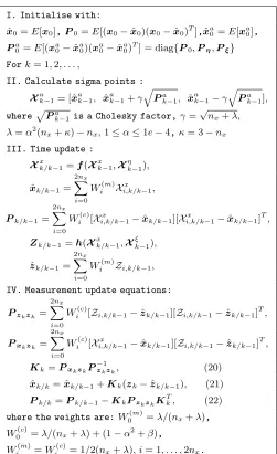
5 An Unscented Kalman Filter for Traffic Flow Estimation
Other algorithms for approximating the posterior state PDF have been introduced. The Unscented Kalman fil-ter (UKF) relies on the unscented transformation (Julier and Uhlmann, 2004; Wan and van der Merwe, 2001), a method for calculating the statistics of a random vari-able which undergoes a nonlinear transformation. Con-sider propagating a random variablex(with dimension
nx) through a nonlinear transformationy=f(x) . As-sume thatxhas mean ˆxand covariance matrix P. To calculate the statistics ofy, a matrixX of 2.nx+1 sigma pointsXiis formed. These sigma points are propagated through the time update. To compute the measurement update step, we propagate these sigma points through the measurement function h and we get transformed pointsZi,k/k−1that form the matrixZk/k−1. Similarly to the Kalman filter, the Kalman gainK, the state esti-mate ˆxand the corresponding covariance matrixP are updated by (20)-(22). The UKF equations are given as Algorithm 3. We implemented the UKF using an aug-mented state vector concatenating the original state and the noise variables:xa
k = (xTk, ηTk, ξ T
k)T (Wan and van der Merwe, 2001). The corresponding matrix with sigma points isXa = ((Xx)T, (Xη)T, (Xξ)T)T. Unlike the PF, the sigma points of the UKF are deterministically chosen so that they exhibit certain properties, e.g. have a given mean and covariance. The UKF is formulated for Gaussian distributions of the noises, whereas the PF has the advantage to work with arbitrary distributions.
6 Particle Filter Performance Evaluation
6.1 Investigations with Synthetic Data
The PF performance is evaluated versus the UKF over of freeway stretch of 4 [km] consisting of eight segments, having periods of congestion. The data are generated by the compositional model (Boel and Mihaylova, 2006) with independent measurement noises for different runs and with different initial state conditions. The conges-tion is due to variaconges-tions in the inflow Qin
k and outflow
Qout
k (shown in Fig. 2) within the period 1.12 h - 1.7 h and due to the fall in the speed vout
Algorithm 3. Unscented Kalman Filter Equations.
I. Initialise with:
ˆ
x0=E[x0],P0=E[(x0−xˆ0)(x0−xˆ0)T],xˆa0=E[xa0],
Pa0=E[(xa0−xˆa0)(xa0−xˆa0)T] = diag{P0,Pη,Pξ}
Fork= 1,2, . . . ,
II. Calculate sigma points :
Xak−1= [ˆx
a k−1, xˆ
a k−1+γ
q
Pak −1, xˆ
a k−1−γ
q
Pak −1],
wherep
Pak−1 is a Cholesky factor,γ= √
nx+λ,
λ=α2(nx+κ)−nx,1≤α≤1e−4,κ= 3−nx
III. Time update :
Xxk/k−1=f(X
x k−1,X
η k−1), ˆ
xk/k−1=
2nx
X
i=0
Wi(m)Xi,k/kx −1,
Pk/k−1=
2nx
X
i=0
Wi(c)[Xi,k/kx −1−xˆk/k−1][X
x
i,k/k−1−xˆk/k−1]
T,
Zk/k−1=h(X
x k/k−1,X
ξ k−1), ˆ
zk/k−1=
2nx
X
i=0
Wi(m)Zi,k/k−1,
IV. Measurement update equations:
Pzkzk=
2nx
X
i=0
Wi(c)[Zi,k/k−1−zˆk/k−1][Zi,k/k−1−zˆk/k−1]
T,
Pxkzk =
2nx
X
i=0
Wi(c)[Xi,k/kx −1−xˆk/k−1][Zi,k/k−1−zˆk/k−1]
T,
Kk=PxkzkP
−1
zkzk, (20)
ˆ
xk/k= ˆxk/k−1+Kk(zk−ˆzk/k−1), (21) Pk/k=Pk/k−1−KkPzkzkK
T
k, (22)
where the weights are:W0(m)=λ/(nx+λ),
W0(c)=λ/(nx+λ) + (1−α2+β),
Wi(m)=Wi(c)= 1/2(nx+λ), i= 1, . . . ,2nx.
outflow boundary conditions (for the state model). The augmented state vector is xk = (xT1,k,xT2,k, . . . ,xT8,k)T, i.e. i = 1,2, . . . ,8, and the measurement vector zs = (zT1,s,zT8,s)T. The per minute aggregated measurements are supplied to the PF and UKF as would be the case with real data. The state prediction is performed also at each intermediate state update time step. We are esti-mating the states of all segments between two measure-ments as one augmented state vector.
1 1.5 2 2.5 3
0 2000 4000 6000 Flows, [veh/h] Time, [h] 1 2
1 1.5 2 2.5 3
[image:7.595.44.295.84.495.2]0 50 100 150 Speed, [km/h] Time, [h] 1 2
Fig. 2. Boundary conditions: 1 - in, 2 - out
The filters’ performance is evaluated by Root mean
square errors(RMSEs)ǫ(ˆxi,k) = [1rPri=1(εi,k)T(εi,k)]1/2,
for the state errors, εi,k =xi,k−xˆi,k, over r indepen-dent Monte Carlo runs, with respect to density, speed and flow. The initial particles for the PF are randomly generated by adding Gaussian noise to the actual states. Table 4 gives the parameters of the state model. The evolution of the flow and speed in time (for one realisa-tion) are given in Figures 3 and 4. We see the backward wave on the evolution of the speed and flow in time. The flow-density and the speed-flow diagrams have the typical bell-shaped forms. The filter performance is evaluated for r = 100 independent Monte Carlo runs. RMSEs calculated withM = 200 for segments 1, 5, and 8 are presented in Fig. 5.
1 1.5 2 2.5 3 0 1000 2000 3000 4000 5000 Flow, [veh/h] Time, [h]
1 1.5 2 2.5 3 0 20 40 60 80 100 120 Speed, [km/h] Time, [h] 8 7 6 5
[image:7.595.307.544.235.425.2]1 2 3 4 5 6 7 8
Fig. 3. Diagrams based on the PF and UKF estimated states
1 1.5 2 2.5 3 0 1000 2000 3000 4000 5000 Flow, [veh/h]
Time, [h] 1 1.5 2 2.5 3
0 20 40 60 80 100 120 Speed, [km/h] Time, [h]
1 2 3 4 5 6 7 8
8 7 6 5
Fig. 4. Diagrams based on the PF and UKF estimated states
We see the influence of the backward wave on these RM-SEs. We observe that the RMSE values in segment 1 are smaller than their values in the intermediate seg-ment 5 (it is also due to the fact that there are no sensor data in this segment). According to these results the PF estimates are more accurate than the UKF estimates. However, the PF complexity is more computationally expensive than the UKF. The complexity of the PF is proportional to the the number of particles, times the dimension of the overall state vector,M.nx, whilst the complexity of the UKF is proportional to the number 2.nx+ 1 of sigma points. Note that nx is equal to the number of segments ntimes the number of states 2 in a segment. We calculated the ratio between the PF and UKF computational time and it is: 2.8 (withM = 100 particles), 5.45 (withM = 200), 15 (withM = 500). The PF more accurate performance compared to the UKF performance can be explained with the fact that the PF approximates the state PDF function, whereas the UKF propagates only the first two moments.
We have also a case with 12.5 km road length (25 seg-ments) where we used the PF with 350 particles and we obtained accuracy comparable to the accuracy with 4
[image:7.595.50.264.614.700.2]kilometers (with 200 particles). In general, the number of necessary particles is increasing with the increased number of states for reaching a certain accuracy, but not very much. It is difficult to characterise in general the PF accuracy and complexity because they highly depend on the road structure and the traffic conditions.
Table 4. Parameters of the traffic model in the PF
vf ree= 120 [km/h] ,vmin= 7.4 [km/h]
ρcrit= 20.89 [veh/km/lane] , ρjam= 180 [veh/km]
α= 0.65 , βk+1= (
0.25, if |ρantic
i+1,k+1−ρi,k+1| ≥2,
0.75, otherwise.
∆ti= 10 [sec],td= 2 [sec] ,Li= 0.5 [km], i= 1, ...,8,
M = 200 particles, td= 2 [sec], Aℓ= 0.01 [km],ℓi= 3
cov{ηSi,k}= (0.03Ni,kvi,k∆tk/Li)
2 [veh]2
cov{ηQi}= 1
2 [veh]2,cov{η
vi}= 3.5
2 [km/h]2
cov{ξQi}= 1
2 [veh]2, cov{ξ
vi}= 5
2 [km/h]2
1 2 3
0 2 4 6
ρ 1
1 2 3
2 4 6
v 1
Root Mean Square Errors
1 2 3
100 200 300 400 500 q1
1 2 3
0 2 4 6
ρ 5
1 2 3
2 4 6
v 5
1 2 3
100 200 300 400 500 q5
1 2 3
0 2 4 6 ρ 8 Time, [h]
1 2 3
2 4 6
v 8
Time, [h]
1 2 3
100 200 300 400 500 q8 Time, [h] UKF PF
Fig. 5. PF and UKF RMSEs of the density (for all lanes) [veh/km], speed [km/h] and flow [veh/h] of segments 1, 5
and 8 (withM = 200 for the PF)
6.2 Application of the Particle Filter to Traffic Data
from E17 Freeway in Belgium
The PF performance has also been evaluated with real data, over a stretch of E17 (between CLOF and CLOA on Fig. 6) freeway between the cities of Ghent and Antwerp, subject to frequent congestions. Measure-ment data are available from video cameras installed at location CLOA, CLOB, CLOD, CLOE, and CLOF, including the total number of vehicles that cross the sensor location during each one minute interval, and the average speed of these vehicles during that one minute interval. We tested the PF and UKF using data mea-sured from September, 2001 from 6.4 [h] a.m. till 10.6 [h] a.m. . This period includes heavy congestions.
TRAVEL DIRECTION
Fig. 6. Schematic representation of the segmentation of the E17 case study freeway. The labels CLOF to CLO1 indicate the locations of the traffic measurement cameras. The verti-cal arrows indicate the location of the used measurements.
Table 5. Model parameters
vf ree= 120 [km/h], vmin= 7.4 [km/h]
βk+1= (
0.3, if |ρantici+1,k+1−ρi,k+1| ≥2,
0.7, otherwise.
L1=L2=L3= 0.6 [km], L4=L5= 0.5 [km]
∆ti= 10 [sec], td= 1.5 [sec], Aℓ= 0.01 [km]
ρcrit= 20.89 [veh/km/lane], ρjam= 180 [veh/km]
M = 100 particles, α= 0.65
Gaussian noisesηSi,k,ηvi,k with covariances: cov{ηSi,k}= (0.035Ni,kvi,k∆tk/Li)
2 [veh]2
cov{ηQi}= 1
2 [veh]2,cov
{ηvi}= 3.5
2[km/h]2,
cov{ξQi}= 1
2 [veh]2,cov
{ξvi}= 5
2[km/h]2
0 50 100 150 200 250
0 1000 2000 3000 4000 5000 6000
Flow, [veh/h]
Density, [veh/km] Estimated with PF
0 50 100 150 200 250
0 1000 2000 3000 4000 5000 6000
Flow, [veh/h]
Density, [veh/km] Estimated with UKF
Fig. 7. Diagrams based on the PF and UKF estimated states
7 8 9 10 0 50 100 150 200 250 ρ , [veh/km]
7 8 9 10 0 20 40 60 80 100 v, [km/h]
7 8 9 10 0
2000 4000 6000
Q, [veh/h]
Fig. 8. PF estimated states (solid line) versus measured states in CLOD (dashed line)
7 8 9 10 0 50 100 150 200 250 ρ , [veh/km]
7 8 9 10 0 20 40 60 80 100 v3 , [km/h]
7 8 9 10 0
2000 4000 6000
Q, [veh/h]
Fig. 9. UKF estimated states (solid line) versus measured states in CLOD (dashed line)
step. The parameters of the models and of the filters are given in Table 5. The filters generate estimates of the state of each segment in a link, and also of the speed and density (and hence also of the flow) at each boundary between segments. Figure 7 presents flow-density dia-grams plotted based on the estimates. The bell-shaped diagram shows nicely that the estimated states indeed have properties as one can expect for traffic data. These estimates of the density, speed, and flow at the bound-aries are compared with the measured data in the inter-mediate segment boundary CLOD (Figs. 8 and 9).
7 Conclusions and Open Issues
This paper formulates the freeway traffic flow estimation within Bayesian recursive framework. A particle filter is developed using traffic and observation models with aggregated variables. The traffic is modelled by a re-cently developed stochastic compositional traffic model with interconnected states of neighbour segments. The PF and UKF performance is investigated and validated by simulated data and by real traffic data from a Bel-gian freeway. Both the results with simulated and real traffic data confirm that the PF provides accurate track-ing performance, better than the UKF. Both the PF and the UKF are suitable methods for real-time traf-fic estimation, and both are easy to implement because of the fact that they do not require linearisation. The estimation approach presented is straightforward, gen-eral, easily executable to freeway and urban networks, with different topologies, with any number of sensors, with regularly or irregularly received data in space and in time. Both methods are suitable for distributed real-isation and parts of them – for parallel computations.
Both the PF and UKF can be used for on-line traffic con-trol strategies, e.g. within the model predictive concon-trol framework (Sun et al., 2003; Hegyi, 2004). One could interpret the results of this paper as follows. Particle fil-tering can successfully estimate and predict the state of all segments of a road link using only observations on the inflow and the outflow of the link. This suggests that it will be possible to obtain efficient filters in large net-works if a few intermediate measurements of the flow are available, and moreover it suggests that these filters for a large network will be nicely decomposable.
Acknowledgments. Financial support by the project
DWTC-CP/40 “Sustainability effects of traffic
manage-ment”, sponsored by the Belgian government is gratefully
acknowledged, as well as by the Belgian Programme on Inter-University Poles of Attraction initiated by the Belgian State, Prime Minister’s Office for Science, Technology and Culture, and in part by projects I-1202/02,I-1205/02 with
the Bulgarian Science Fund. We also thank the “Vlaams
Verkeerscentrum Antwerpen”, Antwerp, Belgium for pro-viding the data used in this study.
References
Boel, R. and Mihaylova, L. (2004). Modelling freeway networks by hybrid stochastic models. In Proc.
IEEE Intelligent Vehicle Symp., pages 182–187.
Boel, R. and Mihaylova, L. (2006). A compositional stochastic model for real-time freeway traffic simu-lation. Transportation Research B, 40(4):319–334. Chen, Z. (2003). Bayesian filtering: From Kalman filters
to particle filters, and beyond.Tech. Rep. McMaster
Univ., Canada.
Daganzo, C. (1994). The cell transmission model: A dy-namic representation of highway traffic consistent with the hydrodynamic theory. Transp. Res. B, 28B(4):269–287.
Doucet, A., Freitas, N., and N. Gordon, E. (2001).
Se-quential Monte Carlo Methods in Practice. New
York: Springer.
Gordon, N., Salmond, D., and Smith, A. (1993). A novel approach to nonlinear/ non-Gaussian Bayesian state estimation. IEE Proc. Radar & Signal Proc., 40:107–113.
Hegyi, A. (2004). Model Predictive Control for
Inte-grating Traffic Control Measures. PhD thesis, Delft
University of Technology, the Netherlands.
Helbing, D. (2002). Traffic and related self-driven many-particle systems.Rev. Modern Phys., 73:1067–1141. Hoogendoorn, S. and Bovy, P. (2001). State-of-the-art of vehicular traffic flow modelling.Journal of Systems Control Engineer — Proceedings of the Institution
of Mechanical Engineers, Part I, 215(14):283–303.
Julier, S. and Uhlmann, J. (2004). Unscented filtering and nonlinear estimation.Proceedings of the IEEE, 92(3):401–422.
Kotsialos, A., Papageorgiou, M., Diakaki, C., Pavlis, Y., and Middelham, F. (2002). Traffic flow modeling of large-scale motorway using the macroscopic model-ing tool METANET. IEEE Transactions on
Intel-ligent Transportation Systems, 3(4):282–292.
Mihaylova, L. and Boel, R. (2004). A particle filter for freeway traffic estimation. InProc. 43rd IEEE Conf.
on Decision and Control, pages 2106–2111.
Papageorgiou, M. and Blosseville, J.-M. (1989). Macro-scopic modelling of traffic flow on the boulevard P´eriph´erique in Paris.Transp. Res. B, 23(1):29–47. Ristic, B., Arulampalam, S., and Gordon, N. (2004). Be-yond the Kalman Filter: Particle Filters for
Track-ing Applications. Artech House.
Sun, X., Mu˜noz, L., and Horowitz, R. (2003). High-way traffic state estimation using improved mixture Kalman filters for effective ramp metering control.
InProc. 42th IEEE Conf. on Dec. and Contr., pages
6333–6338.
Wan, E. and van der Merwe, R. (2001). The Unscented Kalman Filter, Ch. 7: Kalman Filtering and Neural
Networks. Ed. by S. Haykin, pages 221–280. Wiley.
Wang, Y. and Papageorgiou, M. (2005). Real-time freeway traffic state estimation based on extended Kalman filter: a general approach. Transp. Res. B, 39(2):141–167.