promoting access to White Rose research papers
White Rose Research Online
Universities of Leeds, Sheffield and York
http://eprints.whiterose.ac.uk/
This is an author produced version of a paper published in Mechanical Systems and Signal Processing.
White Rose Research Online URL for this paper: http://eprints.whiterose.ac.uk/3533/
Published paper
Linear Parameter Estimation for
Multi-Degree-of-Freedom Nonlinear Systems Using
Nonlinear Output Frequency Response
Functions
Z.K. Peng, Z.Q. Lang, and S. A. Billings
Department of Automatic Control and Systems Engineering, University of Sheffield Mappin Street, Sheffield, S1 3JD, UK
Email: [email protected]; [email protected]; [email protected] Abstract: The Volterra series approach has been widely used for the analysis of nonlinear systems. Based on the Volterra series, a novel concept named Nonlinear Output Frequency Response Functions (NOFRFs) was proposed by the authors. This concept can be considered as an alternative extension of the classical frequency response function for linear systems to the nonlinear case. In this study, based on the NOFRFs, a novel algorithm is developed to estimate the linear stiffness and damping parameters of multi-degree-of-freedom (MDOF) nonlinear systems. The validity of this NOFRF based parameter estimation algorithm is demonstrated by numerical studies.
Nomenclature
x(t), u(t) the output and input of the nonlinear system
( )
X jω ,U(jω) the spectrum of the system output and input )
,..., ( 1 n n
h τ τ the nth order Volterra kernel
) ,..., ( 1 n
n j j
H ω ω the nth order GFRF
) (jω
Gn the nth order NOFRF n
Ω the frequency components of the nth order output of the system subjected to harmonic inputs
Ω the frequency components of the output of the system )
(jω
GnH the nth order NOFRF of the system subjected to harmonic inputs M, K, C the system mass, damping and stiffness matrices
mi, ki, ci the ith mass, damping and stiffness parameter
) (Δ LS
S ,SLD(Δ&) the restoring forces of the nonlinear spring and damper ri, wi (i=1,…,P) the nonlinearity related parameters
) (t
xi , )Xi(jω the displacement and the output frequency response of the ith mass
) ,..., ( 1
) ,
(i j j
h τ τ the jth order Volterra kernel associated to the
ith mass )
(
) ,
( jω
Gil the lth order NOFRF associated to the
ith mass )
(
1
, ω
λini+ j the ratio between the nth NOFRFs of the ith and (i+1)th masses W the vector of the unknown parameters to be estimated
) (
) , 1 (L− Z jω
Γ the term introduced by the nonlinear force NonF for the Zth order
NOFRF.
1 Introduction
Various methods have been developed to estimate the stiffness and damping parameters for linear structures or machines. Most of these are based on modal analysis techniques, which were essentially derived from the Frequency Response Functions (FRFs) [1]-[5]. To tackle the problem with finite element model updating, Arruda and Santos [1] estimated the mechanical parameters via curve fitting for measured frequency response functions using a non-linear least-squares method. Sunder and Ting [2] used the system parameter estimation method to detect the occurrence and location of damage on steel jacket offshore platforms. Also based on the FRFs, Hwang put forward an identification method for stiffness and damping parameters of connections using test data for a structure attached to another structure via connections [3]. Woodgate studied the problem of identifying a positive semi-definite symmetric stiffness matrix for a stable elastic structure from measurements of its displacement in response to some set of static loads [4]. Most recently, Živanović, Pavic and Reynolds [5] described a lively full-scale footbridge from its numerical modelling and dynamic testing. Their work is a successful application of the FRFs to system parameter estimation in practice.
However, there are certain types of qualitative behaviour, which cannot be produced by linear models [6], encountered in engineering, for example, the generation of harmonics and inter-modulation behaviours. In cases where these effects are dominant or significant nonlinear behaviours exist, nonlinear models are required to describe the system, and the linear FRFs are no longer suitable to investigate the system dynamics.
a convenient tool for analyzing nonlinear systems in the frequency domain. If a differential equation or discrete-time model is available for a system, the GFRFs can be determined using the algorithms in [9]~[11]. The GFRFs can be regarded as the extension of the classical frequency response function (FRF) of linear systems to the nonlinear case. So far only a few researchers have addressed the problem of nonlinear system parameter estimation for nonlinear systems using the GFRFs. Lee proposed a straightforward method to estimate the nonlinear system parameters using the GFRFs [12]. Khan and Vyas [13] employed the relationships between higher order GFRFs and first order GFRF to estimate the non-linear parameters. Later, Chatterjee and Vyas [14] further developed this method by using a method of recursive iteration.
In engineering practice, for many mechanical and structural systems, more than one coordinate is needed to sufficiently describe the system dynamics. The result is a MDOF model. In addition, there are considerable mechanical and structural systems that behave nonlinearly just because one or a few components within the system are nonlinear. One well known example is beam structures [15] with breathing cracks, the global nonlinear behaviours of which are caused only by the cracked elements. Such nonlinear MDOF systems can be regarded as locally nonlinear MDOF systems. An important fact is that, for such nonlinear systems, the linear stiffness and damping are still the decisive characteristics which mainly determine the system behaviour. Therefore, a knowledge of the linear stiffness and damping are still of great significance for understanding the whole system dynamical properties.
2. Nonlinear Output Frequency Response Functions
2.1 Nonlinear Output Frequency Response Functions under General Inputs
The definition of NOFRFs is based on the Volterra series theory of nonlinear systems. The Volterra series extends the well-known convolution integral description for linear systems to a series of multi-dimensional convolution integrals, which can be used to represent a wide class of nonlinear systems [8].
Consider the class of nonlinear systems which are stable at zero equilibrium and which can be described in the neighbourhood of the equilibrium by the Volterra series
1
1 1
( ) ( ,..., ) ( ) n
N
n n i i
n i
x t ∞ ∞ h τ τ u t τ τd
−∞ −∞
= =
=
∑
∫ ∫
L∏
− (1) where x(t) and u(t) are the output and input of the system, hn(τ1,...,τn) is the nth order Volterra kernel, and N denotes the maximum order of the system nonlinearity. Lang and Billings [8] derived an expression for the output frequency response of this class of nonlinear systems to a general input. The result is1
1
1 1
1 ,...,
( ) ( ) for 1
( ) ( ,..., ) ( )
(2 )
n
N
n n
n
n n n n i n
i
X j X j
n
X j H j j U j d ω
ω ω ω
ω ω ω
ω ω ω ω σ
π =
−
= + + =
⎧ = ∀
⎪ ⎪ ⎨
⎪ =
⎪⎩
∑
∏
∫
(2)
This expression reveals how nonlinear mechanisms operate on the input spectra to produce the system output frequency response. In (2), (X jω) and U(jω) are the spectrum of the system output and input respectively, Xn(jω) represents the nth order output frequency response of the system,
n j
n n
n
n j j h e d d
H ( ω ,..., ω ) ... (τ ,...,τ ) ωτ ωnτn τ ... τ
1 ) ,..., ( 1
1 11
+ + − ∞
∞ − ∞
∞ −
∫
∫
= (3)
is the nth order Generalised Frequency Response Function (GFRF) [8], and
∫
∏
= +
+ ω ω =
ω
ω σ ω ω
ω
n
n n
i
i n
n j j U j d
H
,..., 1
1
1
) ( ) ,..., ( denotes the integration of
∏
= n
i
i n
n j j U j
H
1
1,..., ) ( )
( ω ω ω over the n-dimensional hyper-plane ω
ω
ω1+L+ n = . Equation (2) is a natural extension of the well-known linear relationship ( ) ( ) ( )
X jω =H jω U jω , where H(jω) is the frequency response function, to the nonlinear case.
input, the output frequencies of system (1) can be determined using the explicit expression derived by Lang and Billings in [8].
Based on the above results for the output frequency response of nonlinear systems, a new concept known as Nonlinear Output Frequency Response Function (NOFRF) was recently introduced by Lang and Billings [16]. The NOFRF is defined as
∫ ∏
∫
∏
= +
+ =
= +
+ =
=
ω ω ω
ω ω
ω ω
ω
σ ω
σ ω ω
ω ω
n n
n n
i
i
n n
i
i n
n
n
d j U
d j U j
j H j
G
,..., 1
,..., 1 1
1 1
) (
) ( ) ,..., ( )
( (4)
under the condition that
0 )
( )
(
,..., 1
1
≠
=
∫ ∏
= + + ω ω = ω
ω σ ω ω
n
n n
i
i
n j U j d
U (5) Notice that Gn(jω) is valid over the frequency range of Un(jω) , which can be determined using the algorithm in [8].
By introducing the NOFRFs Gn(jω), n=1,LN, equation (2) can be written as
1 1
( ) N n( ) N n( ) n( )
n n
X jω X jω G jω U jω
= =
=
∑
=∑
(6) which is similar to the description of the output frequency response for linear systems. The NOFRFs reflect a combined contribution of the system and the input to the system output frequency response behaviour. It can be seen from equation (4) that Gn(jω) depends not only on Hn (n=1,…,N) but also on the input U(jω). For any structure, the dynamical properties are determined by the GFRFs Hn (n= 1,…,N). However, from equation (3) it can be seen that the GFRF is multidimensional [18][19], which makes the GFRFs difficult to measure, display and interpret in practice. Feijoo, Worden and Stanway [20][21] demonstrated that the Volterra series can be described by a series of associated linear equations (ALEs) whose corresponding associated frequency response functions (AFRFs) are easier to analyze and interpret than the GFRFs. According to equation (4), the NOFRF Gn(jω) is a weighted sum of Hn(jω1,..., jωn) overω ω
2.2 Nonlinear Output Frequency Response Functions under Harmonic Inputs Harmonic inputs are pure sinusoidal signals which have been widely used for the dynamic testing of many engineering structures. Therefore, it is necessary to extend the NOFRF concept to the harmonic input case.
When system (1) is subject to a harmonic input
) cos(
)
(t =A ω t+β
u F (7) Lang and Billings [8] showed that equation (2) can be expressed as
1 1
1
1 1
1
( ) ( ) ( , , ) ( ) ( )
2 n n
k kn
N N
n n n k k k k
n n
X j X j H j j A j A j
ω ω ω
ω ω ω ω ω ω
= = + + =
⎛ ⎞
= = ⎜⎜ ⎟⎟
⎝ ⎠
∑
∑
∑
L
L L (8)
where
⎩ ⎨ ⎧ =
0 | | ) (
) ( sign β
ωk A ej k
j A
i
if
{
}
otherwise
, , 1 , 1
,k i n
k F
ki ∈ ω =± = L ω
(9) Defining the frequency components of the nth order output of the system as Ωn, then according to equation (8), the frequency components in the system output can be expressed as
U
nN n1
= Ω =
Ω (10) and Ωn is determined by the set of frequencies
{
k k k F i n}
i
n | , 1, ,
1+L+ =± = L
=ω ω ω ω
ω (11) From equation (11), it is known that if all
n
k
k ω
ω , ,
1 L are taken as −ωF, then ω=−nωF.
If k of these are taken as ωF, then ω =(−n+2k)ωF. The maximal k is n. Therefore the possible frequency components of Xn(jω) are
n
Ω =
{
(−n+2k)ωF,k =0,1,L,n}
(12) Moreover, it is easy to deduce that} , , 1 , 0 , 1 , , ,
{
1
N N
k k F N
n
n L L
U
Ω = =− −= Ω
=
ω (13) Equation (13) explains why some superharmonic components will be generated when a nonlinear system is subjected to a harmonic excitation. In the following, only those components with positive frequencies will be considered.
The NOFRFs defined in equation (4) can be extended to the case of harmonic inputs as
∑
∑
= + + = + + =
ω ω ω ω ω ω
ω ω
ω ω
ω ω
ω
kn k
n kn
k
n n
k k
n
k k
k k
n n
H n
j A j
A
j A j
A j j
H
j G
L L
L
L L
1
1 1
1 1
) ( ) ( 2
1
) ( ) ( ) , , ( 2
1 )
under the condition that
0 ) ( ) ( 2
1 ) (
1
1 ≠
=
∑
= + + ω ω ω
ω ω
ω
kn k
n
k k
n
n j A j A j
A
L
L (15) Obviously, )GnH(jω is only valid over Ωn defined by equation (12). Consequently, the output spectrum (X jω) of nonlinear systems under a harmonic input can be expressed as
1 1
( ) N ( ) N H( ) ( )
n n n
n n
X jω X jω G jω A jω
= =
=
∑
=∑
(16) When k of the n frequencies ofn
k
k ω
ω1,L, are taken as ωF and the remainders are as F
ω
− , substituting equation (9) into equation (15) yields,
β
ω | | ( 2 )
2 1 ) ) 2 (
( k n j n k
n n F
n j n k C A e
A − + = − + (17) Thus )GnH(jω becomes
β
β ω
ω ω
ω ω
) 2 (
) 2 (
| | 2
1
| | ) , , ,
, , ( 2
1 ) ) 2 ( (
k n j n k n n
k n j n k n k
n
F F
k
F F
n n F H
n
e A C
e A C j j
j j
H k
n j G
+ −
+ − −
− −
= +
−
4 4 8 4
4 7 6
L 4
48 4
47 6
L
) , , ,
, ,
(6474L484 64 74L4 84 k n
F F
k
F F
n j j j j
H
− − −
= ω ω ω ω (18) where )Hn(jω1,...,jωn is assumed to be a symmetric function. Therefore, in this case,
) (jω
GnH over the nth order output frequency range Ωn=
{
(−n+2k)ωF,k =0,1,L,n}
is equal to the GFRFHn(jω1,...,jωn) evaluated atω1=L=ωk =ωF, ωk+1 =L=ωn =−ωF,n k=0,L, .
3. The NOFRFs of Locally Nonlinear MDOF Systems
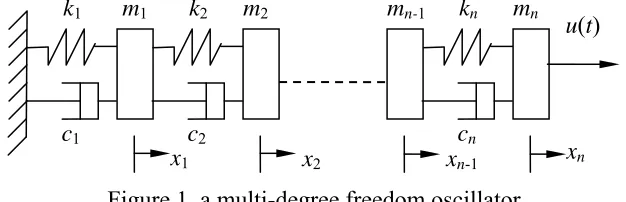
[image:8.612.149.462.530.631.2]The locally nonlinear MDOF systems to be investigated are shown in Figure 1.
Figure 1, a multi-degree freedom oscillator
If all springs and dampers of the systems have linear properties, then the governing motion equation of the MDOF oscillator can be written as
) (t U Kx x C x
M&&+ &+ = (19) where M is the system mass matrix,
mn
kn
mn-1
m2
m1 k2
k1
x1 x2 xn-1 xn
u(t)
⎥ ⎥ ⎥ ⎥
⎦ ⎤
⎢ ⎢ ⎢ ⎢
⎣ ⎡
=
n m m
m
M
L M O M M
L L
0 0
0 0
0 0
2 1
C and K are the system damping and stiffness matrices respectively,
⎥ ⎥ ⎥ ⎥ ⎥ ⎥
⎦ ⎤
⎢ ⎢ ⎢ ⎢ ⎢ ⎢
⎣ ⎡
−
− + −
− + −
− +
=
− −
n n
n n n n
c c
c c c c
c c c c
c c
c
C
0 0
0 0
0 0
1 1 3 3 2 2
2 2
1
L O M
O O
O
M O
L
⎥ ⎥ ⎥ ⎥ ⎥ ⎥
⎦ ⎤
⎢ ⎢ ⎢ ⎢ ⎢ ⎢
⎣ ⎡
−
− + −
− + −
− +
=
− −
n n
n n n n
k k
k k k k
k k k k
k k
k
K
0 0
0 0
0 0
1 1 3 3 2 2
2 2
1
L O M
O O
O
M O
L
x is the displacement, x=(x1,L,xn)', and u(t) is the external force acting on the right end of the oscillator, U(t)=
(
0,L,u(t))
'.Equation (19) forms the basis of the modal analysis method, which is a well-established approach for determining dynamic characteristics of engineering structures. In the linear case, the displacements xi(t) (i=1,L,n) can be expressed as
∫
−+∞∞ −= h t τ u τ dτ
t
xi( ) (i)( ) ( ) (20) where )h(i)(t (i=1,L,n) are the impulse response functions that are determined by equation (19), the Fourier transforms of which are the well-known FRFs of the system. Assume the characteristics of the Lth spring and damper are nonlinear, and the restoring forces )SLS(Δ and SLD(Δ&) of the spring and damper are the polynomial functions of the deformation Δ and its derivative Δ& respectively, e.g.,
∑
= Δ =
Δ P
i i i
LS r
S
1
)
( ,
∑
= Δ =
Δ P
i i i
LD w
S
1
)
( & (21) where P is the degree of the polynomials. Without loss of generality, further assume
n
L≠1, . Then the motion of the oscillator in Figure 1 can be described by equations (22)~(26) as follows.
For the masses that are not connected to the Lth spring and damper, the governing motion equations are
0 )
( )
( 1 2 1 2 2 1 2 1 2 2
1
1x + c +c x −c x + k +k x −k x =
m && & & (22) 0
) (
)
( + 1 − 1− 1 1+ + 1 − 1− 1 1 = + i i+ i i i− i+ i+ i i+ i i i− i+ i+ i
ix c c x cx c x k k x k x k x
m && & & &
(i≠L−1,L) (23) 0
1
1+ − =
−
+ n n n n− n n n n− n
nx c x c x k x k x
0 ) (
) (
) (
) (
2
1 2
1 2
1
1 1
2 1 1 1
1 1
= − +
− +
− −
+ + −
− +
+
∑
∑
= −
= −
− −
− −
− − − −
− −
P
i
i L L i P
i
i L L i L L L L
L L L L L L L L L L L L
x x w x
x r x
c x c
x c c x k x k x k k x m
& & &
&
& &&
(25) For the mass that is connected to the right of the Lth spring and damper, the governing motion equation is
0 ) (
) (
) (
) (
2 1
2 1
1 1 1
1 1
1 1 1
= − −
− −
− −
+ + −
− +
+
∑
∑
= −
= −
+ + −
+ +
+ − +
P
i
i L L i P
i
i L L i L
L L L
L L L L L L L L L L L L
x x w x
x r x
c x c
x c c x k x k x k k x m
& & &
&
& &&
(26) Denote
∑
∑
= −
= −
− +
−
= P
i
i L L i P
i
i L L
i x x r x x
w NonF
2 1 2
1 ) ( )
(& & (27)
}2 } '
0 0 0
0 ⎟⎟
⎠ ⎞ ⎜
⎜ ⎝ ⎛
− =
−
− n L
L
NonF NonF
NF L L (28) Then, the governing motion equation of the locally nonlinear oscillator can be written as
) (t U NF Kx
x C x
M&&+ &+ =− + (29) The systems described by (27)~(29) are typical locally nonlinear MDOF systems. The Lth nonlinear spring and damper components can lead the whole system to behave nonlinearly. Based on the Volterra series theory of nonlinear systems, the relationships between the displacements xi(t) (i=1,L,n) and the input force u(t) of the MDOF systems are
l j
l
l N
j
j j
i
i t h u t d
x( ) (τ ,...,τ ) ( τ ) τ
1 1
1 ) ,
(
∏
∑∫ ∫
= =
∞
∞ −
∞
∞
− −
= L (i=1,L,n) (30) where )h(i,j)(τ1,...,τj is the j
th order Volterra kernel associated to the
ith mass. In the frequency domain, the relationship (30) can be expressed as
∑
∑
= =
=
= N
l
l l
i N
l l i
i j X j G j U j
X
1 ) , ( 1
) ,
( ( ) ( ) ( )
)
( ω ω ω ω (i=1,L,n) (31) where )G(i,l)(jω is the lth order NOFRF associated to the ith mass.
In a recent study by the authors [17], a series of relationships between the NOFRF )
(
) ,
( jω
) ( ) ( ) ( ) ( ) ( ) ( ) , 1 ( ) , ( 1 , ) 2 , 1 ( ) 2 , ( 1 , 2 ω ω ω λ ω ω ω λ j G j G j j G j G j N i N i i i N i i i i + + + + = = = =
L (1≤i≤n−1) (32)
) ( ) ( ) ( ) ( ) ( )
( , 1
) , 1 ( ) , ( ) 1 , 1 ( ) 1 , ( 1 ,
1 ω λ ω
ω ω ω ω λ j j G j G j G j G
j iZi
Z i Z i i i i i + + +
+ = = = (1≤ ≤ −2
L
i ,2≤Z ≤N) (33) and ) ( ) ( ) ( ) ( ) ( )
( , 1
) , 1 ( ) , ( ) 1 , 1 ( ) 1 , ( 1 ,
1 ω λ ω
ω ω ω ω λ j j G j G j G j G
j iZi
Z i Z i i i i i + + +
+ = ≠ = ( −1≤ ≤ −1
n i
L ,2≤Z ≤N) (34) where
(
)
(
) (
)
[
− + − + + + − +]
⎝⎛⎜⎜ + Λ + ⎞⎠⎟⎟= + + + + − + − + + + 1 1 1 , 1 , 1 1 , 1 2 1 1 1
, 1 ( )
) ( 1 ) ( 1 ) ( i i i i Z i i i i Z i i i i Z i i i i i Z k jc j k k j c c j j m k jc j ω ω ω λ ω ω λ ω ω ω λ
(1≤i≤n−1,1≤Z ≤N) (35) with 0λ0,1(ω)=
Z , ⎪ ⎪ ⎪ ⎪ ⎩ ⎪⎪ ⎪ ⎪ ⎨ ⎧ = ≥ Γ − = ≥ Γ − − ≠ = = Λ + − − + and 2 for ) ( ) ( , 1 and 2 for ) ( ) ( , 1 or 1, for 0 ) ( ) , 1 ( ) , 1 ( ) , ( ) , 1 ( 1 , L i Z j G j L i Z j G j L L i Z j Z L Z L Z L Z L i i Z ω ω ω ω
ω (36)
and Γ(L−1,Z)(jω) is a term introduced by the nonlinear force NonF for the Zth order NOFRF. As the form of Γ(L−1,Z)(jω) will not play crucial role in this study, its explicit expression will not be given.
4. The Linear Stiffness and Damping Estimation Method
Based on the results in Section 3, a novel method is developed in this section to estimate the linear stiffness and damping parameters for locally nonlinear MDOF systems. This method requires that the masses mi, (i=1,L,n) of the systems are known a priori. This is a reasonable assumption since the mass distribution of a mechanical structure or machine can usually be predetermined during the design stage and will not change significantly with the change of the structure’s or machine’s conditions even after years’ operation. In addition, the mass distribution can be easily obtained using the FE method or other methods.
Consider Z= 1 in (35), it is known that
(
)
(
)
(
)
(
)
, 1 21 1 1 , 1 1 , 1 , 1 1 1 1 , 1 1 , 1 , 1 1 ) ( 1 ) ( ) ( ) ( 1 1 ) ( ) ( ) ( 1 ω ω λ ω λ ω λ ω λ ω λ ω ω λ ω λ ω j m k j k j j c j j c j j j i i i i i i i i i i i i i i i i i i i + + + + − + + + − = − + − + − + −
(1≤i≤n−1) (37)
(
1 ( ))
( ) )( , 1
1 , 1 1 1 , , 1
1 jω λ jω λ jω
i i i i i i
i− + = − − +
Π , ( ) , 1( ) 1
1 1
,
1 = −
Π + ω λ + ω
j j ii i i
(
)
(
)
(
)
(
)
(
)
(
)
(
)
(
)
⎟⎟⎠⎞ ⎜⎜ ⎝ ⎛ Π Π Π Π Π Π − Π Π − = Φ + + + − + − + + + − + − + − ) ( Im ) ( Re ) ( Im ) ( Re ) ( Re ) ( Im ) ( Re ) ( Im ) ( 1 , 1 1 , 1 1 , , 1 1 1 , , 1 1 1 , 1 1 , 1 1 , , 1 1 1 , , 1 1 1 , , 1 1 ω ω ω ω ω ω ω ω ω ω ω ω ω j j j j j j j j j i i i i i i i i i i i i i i i i i i i i i i i and[
]
Ti i i i i i k c k c
W ,+1 = +1 +1 Equation (37) can then be written as
(
)
(
)
⎥ ⎦ ⎤ ⎢ ⎣ ⎡ =Φ− + + ++
2 1 , 1 2 1 , 1 1 , 1 , , 1 1 ) ( Im ) ( Re ) ( ω ω λ ω ω λ ω j m j m W
j ii
i i i i i i i i
i (1≤ ≤ −1
n
i ) (38) where i,i+1
W is the parameter vector to be estimated.
Consider Z = 2 in (35), an equation similar to (38) can be obtained for i≠L−1,Las
(
)
(
)
⎥ ⎦ ⎤ ⎢ ⎣ ⎡ =Φ− + + ++
2 1 , 2 2 1 , 2 1 , 1 , , 1 2 ) ( Im ) ( Re ) ( ω ω λ ω ω λ ω j m j m W
j ii
i i i i i i i i
i (
L L i n
i 1,and 1,
1≤ ≤ − ≠ − ) (39) For i=L-1 and i=L, the extra terms introduced by the nonlinear force NonF should be taken into account. When i=L-1, the result is
(
)
(
) (
)
1, 1 2 1 , 2 2 , 1 2 1 , 1 2 1 , 2
2 ( ) ( ) ( ) 1 1 ( ) ( )
1− − − − − + − − + − L− L− L− L L− L L L L L L L L k j j c j j c j j
jω λ ω λ ω ω λ ω λ ω λ ω
(
)
1, 22 1 , 1 2 , 1
2 ( ω) 1 ( ω) λ ( ω)ω
λ j k j mL L L j
L L L L L − − −
− − −Λ =
+ (40) which can further be written as
(
)
(
)
⎥ ⎦ ⎤ ⎢ ⎣ ⎡ = ⎥ ⎥ ⎥ ⎦ ⎤ ⎢ ⎢ ⎢ ⎣ ⎡ Λ Λ ⎟⎟ ⎠ ⎞ ⎜⎜ ⎝ ⎛ − − Φ − − − − − − − − − 2 , 1 2 1 2 , 1 2 1 , 1 2 , 1 2 , 1 , 1 , 2 2 ) ( Im ) ( Re )) ( Im( )) ( Re( 1 0 0 1 ) ( ω ω λ ω ω λ ω ω ω j m j m j j Wj L L
L L L L L L L L L L L L
L (41)
For i=L, the result is
(
)
(
)
⎥ ⎦ ⎤ ⎢ ⎣ ⎡ = ⎥ ⎥ ⎥ ⎦ ⎤ ⎢ ⎢ ⎢ ⎣ ⎡ Λ Λ ⎟⎟ ⎠ ⎞ ⎜⎜ ⎝ ⎛ − −Φ ++
+ + + + − 2 1 , 2 2 1 , 2 1 , 2 1 , 2 1 , 1 , , 1 2 ) ( Im ) ( Re )) ( Im( )) ( Re( 1 0 0 1 ) ( ω ω λ ω ω λ ω ω ω j m j m j j W
j LL
L L L L L L L L L L L L
L (42)
According to equation (36), it can be known
) ( ) ( ) ( ) ( )
( , 1
2 ) 2 , 1 ( ) 2 , ( , 1 2 1 ,
2 λ ω
ω ω ω ω j j G j G j
j LL
L L L L L L + + − + − = − = Λ Λ (43) Substituting equation (43) into equation (42) yields
(
)
(
)
(
)
(
)
⎥⎥⎥ ⎦ ⎤ ⎢ ⎢ ⎢ ⎣ ⎡ Λ Λ ⎟⎟ ⎠ ⎞ ⎜⎜ ⎝ ⎛ − Φ − − + + + + + + − )) ( Im( )) ( Re( ) ( Re ) ( Im ) ( Im ) ( Re ) ( , 1 2 , 1 2 1 , 1 , 2 1 , 2 1 , 2 1 , 2 1 , , 1 2 ω ω ω λ ω λ ω λ ω λ ω j j W j j j j j L L L L L L L L L L L L L L L L L(
)
(
)
⎥ ⎦ ⎤ ⎢ ⎣ ⎡= , ++1 2
2 2 1 , 2 ) ( Im ) ( Re ω ω λ ω ω λ j m j m L L L L L
When a sinusoidal input of frequency ωF is used to excite the system, considering ) ( 1 , 1 F i i jω
λ + and , 1( 2 )
2 F
i i
j ω
λ + , equations (38), (39), (41) and (44) can be written as
(
)
(
)
⎥ ⎦ ⎤ ⎢ ⎣ ⎡ =Φ− + + ++
2 1 , 1 2 1 , 1 1 , 1 , , 1 1 ) ( Im ) ( Re ) ( F F i i i F F i i i i i F i i i j m j m W j ω ω λ ω ω λ
ω (1≤i≤n−1) (45)
(
)
(
)
⎥ ⎦ ⎤ ⎢ ⎣ ⎡ =Φ− + + ++
2 1 , 2 2 1 , 2 1 , 1 , , 1 2 ) 2 ( Im 4 ) 2 ( Re 4 ) 2 ( F F i i i F F i i i i i F i i i j m j m W j ω ω λ ω ω λ
ω (1≤i≤n−1,andi≠ L−1,L) (46)
(
)
(
)
⎥ ⎦ ⎤ ⎢ ⎣ ⎡ = ⎥ ⎥ ⎥ ⎦ ⎤ ⎢ ⎢ ⎢ ⎣ ⎡ Λ Λ ⎟⎟ ⎠ ⎞ ⎜⎜ ⎝ ⎛ Φ − − − − − − − − − 2 , 1 2 1 2 , 1 2 1 , 1 2 , 1 2 , 1 , 1 , 2 2 ) 2 ( Im 4 ) 2 ( Re 4 )) 2 ( Im( )) 2 ( Re( 1 0 0 1 ) 2 ( F F L L L F F L L L F L L F L L L L F L L L j m j m j j W j ω ω λ ω ω λ ω ωω (47)
(
)
(
)
(
)
(
)
⎥⎥⎥ ⎦ ⎤ ⎢ ⎢ ⎢ ⎣ ⎡ Λ Λ ⎟⎟ ⎠ ⎞ ⎜⎜ ⎝ ⎛ − Φ − − + + + + + + − )) 2 ( Im( )) 2 ( Re( ) 2 ( Re ) 2 ( Im ) 2 ( Im ) 2 ( Re ) 2 ( , 1 2 , 1 2 1 , 1 , 2 1 , 2 1 , 2 1 , 2 1 , , 1 2 F L L F L L L L F L L F L L F L L F L L F L L L j j W j j j j j ω ω ω λ ω λ ω λ ω λ ω(
)
(
)
⎥ ⎦ ⎤ ⎢ ⎣ ⎡= , ++1 2
2 2 1 , 2 ) 2 ( Im 4 ) 2 ( Re 4 F F L L L F F L L L j m j m ω ω λ ω ω λ (48) Consider ))Re( 1, ( 2
2 F
L L
j ω
−
Λ and ))Im( 1, ( 2
2 F
L L
j ω
−
Λ as unknown parameters to be estimated, then there are totally 2n+2 parameters to be estimated in equations (45)~(48). There are clearly 4(n-1) equations in total in (45)~(48), and, obviously, when n≥3, the number of equations is sufficient to estimate the unknown parameters.
Denote
[
]
Tn n L L F L L F L L
L-L k j j c k c k
c k c
W = 1 1L −1 1 Re(Λ2−1, ( 2ω )) Im(Λ2−1, ( 2ω )) L and
(
)
(
)
(
)
(
)
[
n n]
TZ n n n Z n Z Z Z j m j m j m j m j ) ( Im ) ( Im ) ( Im ) ( Re ) ( , 1 1 , 1 1 2 , 1 1 2 , 1 1
2 λ ω λ ω λ ω λ ω
ω ω − − − − = Β L
then equations (45)~(48) can be assembled in the following form
⎥ ⎦ ⎤ ⎢ ⎣ ⎡ = ⎟⎟ ⎠ ⎞ ⎜⎜ ⎝ ⎛ Φ Φ ) 2 ( ) ( ) 2 ( ) ( 2 1 2 1 F F F F j B j B W j j ω ω ω ω (49) where both Φ1(jωF) and Φ2(j2ωF) are a 2(n−1)×(2n+2) matrix that can be constructed using a similar procedure given in Appendix 1.
From equation (49), a Least Square based approach can be used to estimate the parameters in W as below
Equation (50) provides a simple way to estimate the linear stiffness and damping coefficients for a locally nonlinear MDOF system from the system NOFRFs. This algorithm requires the information of the 1st and 2nd order NOFRFs under sinusoidal inputs, which can readily be evaluated using an effective algorithm developed in [16] from the system input-output data.
The linear parameter estimation algorithm can be summarized as the following procedures:
Step 1: Estimate G(i,1)(jωF) and G(i,2)(j2ωF)(1≤i≤n) under sinusoidal inputs using the algorithm developed in [16].
Step 2: Calculate , 1( )
1 F
i i
jω
λ + and , 1( 2 )
2 F
i i
j ω
λ + (1≤ ≤ −1
n
i ).
Step 3: Calculate 1,, 1( ω) j i i i Z
+ −
Π , ), 1( ω
j i i Z
+
Π , (1≤i≤n−1, Z = 1, 2).
Step 4: Construct matrixes Φ1(jωF) and Φ2(j2ωF)using the method in Appendix 1. Step 5: Estimate the linear parameters using equation (50).
It is worth pointing out that although the algorithm above can only be used to determine the system linear parameters, the results themself are still of great significance in engineering system analysis such as, for example, in the modal analysis of MDOF systems. In addition the algorithm also provides a premise for the identification of all system characteristic parameters. It can be observed that the term Γ(L−1,Z)(jω) in (36) is related to the system nonlinear parameters. This provides a basis for the system nonlinear parameter estimation. Generally, Γ(L−1,N)(jNωF) can be expressed as
) ( ) , , ( )
( ) , , ( )
( 1,
) , ( )
( ,
1 ) 2 , ( 2
2 ) 2 ( )
, 1
( F
L L
N N F N N N F
L L N F F
N
L jNω Q r w ω F jω Q r w ω F jω
− −
− = + +
Γ L (51)
where )Q(i)(ri,wi,ωF (2≤i≤N) are the functions which only depend on the nonlinear parameters ri and wiand driving frequencyωF , ( )
, 1
) ,
( F
L L
i
N j
F − ω (2≤i≤N−1) depend on both the linear parameters and the nonlinear parameters rl and wl, )(2≤l≤N−i+1 , and
) (
, 1
) ,
( F
L L
N
N j
F − ω only depends on the system linear parameters. According to equation (51), an effective method for the estimation of both the system linear and nonlinear parameters
with the linear parameter estimation using the above algorithm as the first step can be developed. Because of space limitations, this work will be reported in details in a subsequent paper.
5 Numerical Study
the damping is assumed to be proportional damping, e.g., C=μK .The values of the system parameters are
1
6
1 = =m =
m L , r1=k1 =k2 =k3 =3.6×10⁴, k4 =k5 =k6 =0.8k1, 01
. 0 =
μ , 2
1
2 0.8 r
r = × , r3 =0.4×r13, w1 =μr1, w2 =0 and the input is a harmonic force, u(t)= Asin(2π×20t).
If only the NOFRFs up to the 4th order are considered, according to equations (16) and (17), the frequency components of the outputs of the 6 masses can be written as
) ( ) ( )
( ) ( )
( (,1) 1 (,3) F 3 F H
i F F
H i F
i j G j U j G j U j
X ω = ω ω + ω ω
) 2 ( ) 2 ( )
2 ( ) 2 ( )
2
( (,2) 2 (,4) F 4 F H
i F F
H i F
i j G j U j G j U j
X ω = ω ω + ω ω
( 3 ) (,3)( 3 F) 3( 3 F)
H i F
i j G j U j
X ω = ω ω
) 4 ( ) 4 ( )
4
( (,4) F 4 F H
i F
i j G j U j
X ω = ω ω (i=1,L,6) (52) From equation (52), it can be seen that two different inputs with the same waveform but different strengths are sufficient to estimate the NOFRFs up to 4th order. This is the basic principle of the algorithm proposed in [16] for the evaluation of the NOFRFs. Therefore, in this numerical study, two different inputs are used, A=0.8 and A=1.0 respectively. The simulation studies were conducted using a fourth-order Runge–Kutta method to obtain the forced responses of the system. The evaluated results of 1 ( F)
H j
G ω , )G3H(jωF , )
2 (
2 F
H j
G ω and G4H(j2ωF)of the six different masses are given in Table 1. From the evaluated NOFRFs given in Table 1, , 1( )
1 F
i i
jω
λ + , ), 1(
3 F
i i
jω
λ + , , 1( 2 )
2 F
i i
j ω
λ + and
) 2 (
1 ,
4 F
i i
j ω
λ + (
i=1,2,3,4,5) can be evaluated using equations (32), (33) and (34). Moreover, the theoretical values of , 1( )
1 F
i i
jω
λ + , ), 1(
3 F
i i
jω
λ + , ), 1( 2
2 F
i i
j ω
λ + and , 1( 2 )
4 F
i i
j ω
λ +
(i=1,2,3,4,5) can also be calculated using the method in [17]. Both the evaluated and theoretical values of , 1( )
1 F
i i
jω
λ + , ), 1(
3 F
i i
jω
λ + , , 1( 2 )
2 F
i i
j ω
λ + and , 1( 2 )
4 F
i i
j ω
λ + (
i=1,2,3,4,5) are given in Tables 2 and Table 3. The results in Table 2 and Table 3 clearly show that properties (32)~(34) are tenable. Obviously, , 1( )
1 F
i i
jω
λ + ≠ , 1( )
3 F
i i
jω λ + for
[image:15.612.97.516.542.706.2]i=3, 4, 5. Table 1, the evaluated results of 1 ( F)
H j
G ω , )G3H(jωF , )G2H(j2ωF and G4H(j2ωF) )
(
1 F
H j G ω
(×10-6)
) (
3 F
H j
G ω
(×10-7)
) 2 (
2 F
H j
G ω (×10-8)
) 2 (
4 F
H j
G ω (×10-8)
Mass1 -3.5291+6.0326i 1.2996 -2.3216i 2.9244-12.3188i -2.9300 -1.4749i
Mass2 -7.7472+10.2849i 2.8744-3.9706i 12.5722-19.9209i -4.2684-4.3621i
Mass3 -12.8459+11.1323i 4.8088-4.3299i 31.2120-15.1678i -1.9539-8.7759i
Mass4 -19.4063+6.3260i -1.7437+2.4212i -31.6321+11.0973i 0.9027+ 8.6380i
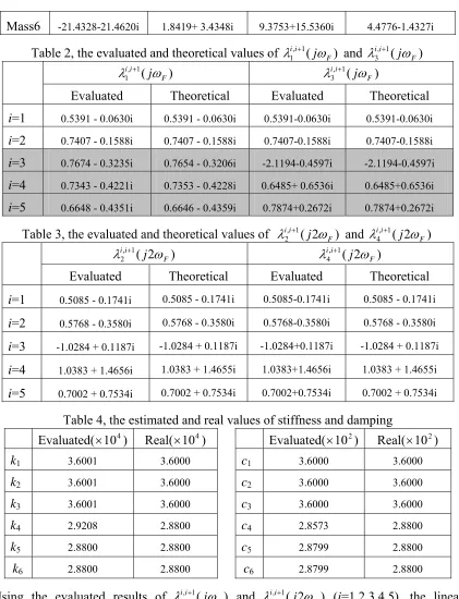
Mass6 -21.4328-21.4620i 1.8419+ 3.4348i 9.3753+15.5360i 4.4776-1.4327i
Table 2, the evaluated and theoretical values of , 1( )
1 F
i i
jω
λ + and , 1( )
3 F
i i
jω λ +
) (
1 ,
1 F
i i
jω
λ + , 1( )
3 F
i i
jω λ +
Evaluated Theoretical Evaluated Theoretical
i=1 0.5391 - 0.0630i 0.5391 - 0.0630i 0.5391-0.0630i 0.5391-0.0630i
i=2 0.7407 - 0.1588i 0.7407 - 0.1588i 0.7407-0.1588i 0.7407-0.1588i
i=3 0.7674 - 0.3235i 0.7654 - 0.3206i -2.1194-0.4597i -2.1194-0.4597i
i=4 0.7343 - 0.4221i 0.7353 - 0.4228i 0.6485+ 0.6536i 0.6485+0.6536i
[image:16.612.96.516.67.273.2]i=5 0.6648 - 0.4351i 0.6646 - 0.4359i 0.7874+0.2672i 0.7874+0.2672i
Table 3, the evaluated and theoretical values of , 1( 2 )
2 F
i i
j ω
λ + and , 1( 2 )
4 F
i i
j ω λ +
) 2 (
1 ,
2 F
i i
j ω
λ + , 1( 2 )
4 F
i i
j ω λ +
Evaluated Theoretical Evaluated Theoretical
i=1 0.5085 - 0.1741i 0.5085 - 0.1741i 0.5085-0.1741i 0.5085 - 0.1741i
i=2 0.5768 - 0.3580i 0.5768 - 0.3580i 0.5768-0.3580i 0.5768 - 0.3580i
i=3 -1.0284 + 0.1187i -1.0284 + 0.1187i -1.0284+0.1187i -1.0284 + 0.1187i
i=4 1.0383 + 1.4656i 1.0383 + 1.4655i 1.0383+1.4656i 1.0383 + 1.4655i
i=5 0.7002 + 0.7534i 0.7002 + 0.7534i 0.7002+0.7534i 0.7002 + 0.7534i
Table 4, the estimated and real values of stiffness and damping
Evaluated(×104) Real(×104) Evaluated(×102) Real(×102)
k1 3.6001 3.6000 c1 3.6000 3.6000
k2 3.6001 3.6000 c2 3.6000 3.6000
k3 3.6001 3.6000 c3 3.6000 3.6000
k4 2.9208 2.8800 c4 2.8573 2.8800
k5 2.8800 2.8800 c5 2.8799 2.8800
k6 2.8800 2.8800 c6 2.8799 2.8800
Using the evaluated results of , 1( )
1 F
i i
jω
λ + and , 1( 2 )
2 F
i i
j ω
λ + (
i=1,2,3,4,5), the linear stiffness and damping can be estimated by the method proposed in the previous section, and the results are given in Table 4. It can be seen that the estimated results match the theoretical results very well except a slightly difference for k4 and c4. This difference
6 Conclusions and Remarks
A new method for the estimation of the linear stiffness and damping parameters of locally nonlinear MDOF systems has been developed. This method is based on the concept of Nonlinear Output Frequency Response Functions (NOFRFs) which were derived from the Volterra series approach of nonlinear systems. This method assumes that the system masses and the position of the system nonlinear component are known priori. The masses can be readily obtained at the system design stage. The position of the nonlinear component can be determined using directly the relationships (32)~(34) [17], which can also be applied to detect the crack position in beams or structures. From these results, all linear stiffness and damping parameters of a nonlinear MDOF system can be estimated using the proposed method directly using the system input-output test data, which are of great engineering significance such as, e.g., in system modal analysis. In addition, although the method is demonstrated on the particular case where the linear oscillators are coupled in series and fixed at one end while excited in the other end, this method can be directly applied (without any modification) to the cases where the excitation force is acting at any position of the system, not only limited to the end.
It is worth pointing out that the present study also provides a necessary basis for the identification of all characteristic parameters for the considered MDOF systems. With the algorithm proposed in this paper as the first step, an effective method can be developed to determine both the linear and nonlinear parameters of the MDOF systems. Because of space limitations, this method will be reported in details in a subsequent paper.
Appendix 1: Construction of Φ1(jωF) and Φ2(j2ωF)
The construction of Φ1(jωF) using this procedure is given as below.
For 1≤i≤L−2, i.e., the first 2(L-2) rows of Φ1(jωF),
⎪ ⎩ ⎪ ⎨ ⎧ = + + − Φ Φ = + − − Φ = − − Φ + − 0 ) 2 2 : 3 2 , 2 : 1 2 )( ( ) ( ) 2 2 : 1 2 , 2 : 1 2 )( ( 0 ) 2 2 : 1 , 2 : 1 2 )( ( 1 1 , , 1 1 1 1 n i i i j j i i i i j i i i j F F i i i F F ω ω ω ω
(1≤i≤L−2) (A-1)
For i= L-1,
⎪ ⎪ ⎩ ⎪ ⎪ ⎨ ⎧ = + + − − − − Φ ⎟⎟ ⎠ ⎞ ⎜⎜ ⎝ ⎛ Φ Φ = + − − − − − −
Φ Φ − − − − − =
− − 0 ) 2 2 : 5 ) 1 ( 2 ), 1 ( 2 : 1 ) 1 ( 2 )( ( ) ( 0 0 0 0 ) ( ) 4 ) 1 ( 2 : 1 ) 1 ( 2 ), 1 ( 2 : 1 ) 1 ( 2 )( ( 0 ) 2 ) 1 ( 2 : 1 ), 1 ( 2 : 1 ) 1 ( 2 )( ( 1 1 , 1 1 , 1 1 1 n L L L j j j L L L L j L L L j F F L Right F L Left F F ω ω ω ω ω (A-2) where
(
)
(
)
(
)
(
)
⎟⎟⎠⎞ ⎜⎜ ⎝ ⎛ Π Π Π Π − =Φ − −− −− −− −−
) ( Im ) ( Re ) ( Re ) ( Im )
( 2, 1, 2, 1,
, 1 , 2 , 1 , 2 1
, ω ω ω
ω ω ω ω j j j j
j L L L
Z L L L Z L L L Z L L L Z L Left
Z (A-3)
(
)
(
)
(
)
(
)
⎟⎟⎠⎞ ⎜⎜ ⎝ ⎛ Π Π Π Π − =Φ − −− −−
) ( Im ) ( Re ) ( Re ) ( Im )
( 1, 1,
, 1 ,
1 1
, ω ω ω
ω ω ω ω j j j j
j L L
Z L L Z L L Z L L Z L Right
Z (A-4) For i=L,
⎪ ⎪ ⎩ ⎪⎪ ⎨ ⎧ = + + − − − − Φ ⎟⎟ ⎠ ⎞ ⎜⎜ ⎝ ⎛ Φ = + − − Φ = − − Φ + − 0 ) 2 2 : 5 ) 1 ( 2 ), 1 ( 2 : 1 ) 1 ( 2 )( ( ) ( 0 0 0 0 ) 4 2 : 1 2 , 2 : 1 2 )( ( 0 ) 2 2 : 1 , 2 : 1 2 )( ( 1 1 , , 1 1 1 1 n L L L j j L L L L j L L L j F F L L L F F ω ω ω ω (A-5)
For L<i≤n−1
⎪ ⎩ ⎪ ⎨ ⎧ = + + − Φ Φ = + + − Φ = − Φ + − 0 ) 2 2 : 5 2 , 2 : 1 2 )( ( ) ( ) 4 2 : 1 2 , 2 : 1 2 )( ( 0 ) 2 : 1 , 2 : 1 2 )( ( 1 1 , , 1 1 1 1 n i i i j j i i i i j i i i j F F i i i F F ω ω ω ω
(L<i≤n−1) (A-6)
⎪ ⎪ ⎩ ⎪ ⎪ ⎨ ⎧ = + + − − − − Φ ⎟⎟ ⎠ ⎞ ⎜⎜ ⎝ ⎛ Φ − − Φ = + − − − − − −
Φ Φ − − − − − =
− − 0 ) 2 2 : 5 ) 1 ( 2 ), 1 ( 2 : 1 ) 1 ( 2 )( 2 ( ) 2 ( 1 0 0 1 ) 2 ( ) 4 ) 1 ( 2 : 1 ) 1 ( 2 ), 1 ( 2 : 1 ) 1 ( 2 )( 2 ( 0 ) 2 ) 1 ( 2 : 1 ), 1 ( 2 : 1 ) 1 ( 2 )( 2 ( 2 1 , 2 1 , 2 2 2 n L L L j j j L L L L j L L L j F F L Right F L Left F F ω ω ω ω ω (A-7)
and for i=L
(
)
(
)
(
)
(
)
⎪ ⎪ ⎪ ⎩ ⎪⎪ ⎪ ⎨ ⎧ = + + − − − − Φ ⎟⎟ ⎠ ⎞ ⎜⎜ ⎝ ⎛ Φ − = + − −Φ Φ − − =
+ − + + + + 0 ) 2 2 : 5 ) 1 ( 2 ), 1 ( 2 : 1 ) 1 ( 2 )( 2 ( ) 2 ( ) 2 ( Re ) 2 ( Im ) 2 ( Im ) 2 ( Re ) 4 2 : 1 2 , 2 : 1 2 )( 2 ( 0 ) 2 2 : 1 , 2 : 1 2 )( 2 ( 2 1 , , 1 2 1 , 2 1 , 2 1 , 2 1 , 2 2 2 n L L L j j j j j j L L L L j L L L j F F L L L F L L F L L F L L F L L F F ω ω ω λ ω λ ω λ ω λ ω ω (A-8)
Acknowledgements
The authors gratefully acknowledge the support of the Engineering and Physical Science Research Council, UK, for this work.
References
1. J.R.F. Arruda, J.M.C. Santos, Mechanical joint parameter estimation using frequency response functions and component mode synthesis, Mechanical Systems and Signal Processing7 (1993) 493–508
2. S. S. Sunder, S. K. Ting, Flexibility monitoring of offshore platforms, Applied Ocean Research,7(1985) 14-23
3. H.Y. Huang, Identification techniques of structure connection parameters using frequency response functions. Journal of Sound and Vibration. 212 (1998)469-479 4. K.G.Woodgate, Effcient stiffness matrix estimation for elastic structures. Computers
and Structures, 69 (1998)79-84
5. S Živanović, A Pavic, P. Reynolds, Modal testing and FE model tuning of a lively footbridge structure.Engineering Structures, 28 (2006)857-868
6. R.K. Pearson, Discrete Time Dynamic Models. Oxford University Press, 1994 7. K. Worden, G. Manson, G.R. Tomlinson, A harmonic probing algorithm for the
multi-input Volterra series. Journal of Sound and Vibration201(1997) 67-84 8. Z. Q. Lang, S. A. Billings, Output frequency characteristics of nonlinear system,
International Journal of Control 64 (1996) 1049-1067.
10.S.A. Billings, J.C. Peyton Jones, Mapping nonlinear integro-differential equations into the frequency domain, International Journal of Control 52(1990) 863-879. 11.J.C. Peyton Jones, S.A. Billings, A recursive algorithm for the computing the
frequency response of a class of nonlinear difference equation models. International Journal of Control50 (1989) 1925-1940.
12.G.M. Lee, Estimation of non-linear system parameters using higher-order frequency response functions. Mechanical Systems and Signal Processing11 (1997) 219-228. 13.A. A. Khan, N. S. Vyas, Non-liner Parameter estimation using Volterra and Wiener
theories. Journal of Sound and Vibration,221 (1999)805-821
14.A Chatterjee, N. S. Vyas.Non-linear parameter estimation with Volterra series using the method of recursive iteration through harmonic probing. Journal of Sound and Vibration, 268 (2003) 657-678
15.T.G. Chondros, A.D. Dimarogonas, J. Yao, Vibration of a beam with breathing crack, Journal of Sound and Vibration, 239 (2001) 57-67
16.Z. Q. Lang, S. A. Billings, Energy transfer properties of nonlinear systems in the frequency domain, International Journal of Control78 (2005) 354-362.
17.Z.K. Peng, Z.Q. Lang, and S. A. Billings, Nonlinear Output Frequency Response Functions of MDOF Systems with Multiple Nonlinear Components, International Journal of Non-Linear Mechanics. (2007, to appear)
18.H. Zhang, S. A. Billings, Analysing non-linear systems in the frequency domain, I: the transfer function, Mechanical Systems and Signal Processing7 (1993) 531-550. 19.H. Zhang, S. A. Billings, Analysing nonlinear systems in the frequency domain, II:
the phase response, Mechanical Systems and Signal Processing8 (1994) 45-62. 20.J. A. Vazquez Feijoo, K. Worden, R. Stanway, Associated Linear Equations for
Volterra operators, Mechanical Systems and Signal Processing 19 (2005)57-69. 21.J. A. Vazquez Feijoo, K. Worden. R. Stanway, System identification using associated
linear equations, Mechanical Systems and Signal Processing 18 (2004)431-455. 22.X.J. Jing, Z.A. Lang, S.A. Billings,New bound characteristics of NARX model in the
frequency domain. International Journal of Control80 (2007): 140-149
23.S.A. Billings, Z.Q. Lang,A bound for the magnitude characteristics of nonlinear output frequency response functions .1. Analysis and computation. International Journal of Control, 65(1996): 309-328
25.A Chatterjee, N. S. Vyas, Convergence analysis of Volterra series response of nonlinear systems subjected to harmonic excitation. Journal of Sound and Vibration,
236 (2006) 339-358
26.I. W. Sandberg, Bounds for Discrete-Time Volterra Series Representations, IEEE Transactions on Circuits and Systems-I: Fundamental Theory and Applications, 46 (1999): 135-139
27.L. Liu, J.P. Thomas, E.H. Dowell, P. Attar and K.C. Hall, A comparison of classical and high dimensional harmonic balance approaches for a Duffing oscillator,Journal of Computational Physics.215 (2006): 298-320.