Time-distance analysis of the emerging active region NOAA 10790

This is a repository copy of

Time-distance analysis of the emerging active region NOAA

10790

.

White Rose Research Online URL for this paper:

http://eprints.whiterose.ac.uk/10478/

Article:

Thompson, M.J. and Zharkov, S. (2008) Time-distance analysis of the emerging active

region NOAA 10790. Solar Physics, 251 (1-2). pp. 369-380. ISSN 1573-093X

https://doi.org/10.1007/s11207-008-9239-z

Reuse

Unless indicated otherwise, fulltext items are protected by copyright with all rights reserved. The copyright exception in section 29 of the Copyright, Designs and Patents Act 1988 allows the making of a single copy solely for the purpose of non-commercial research or private study within the limits of fair dealing. The publisher or other rights-holder may allow further reproduction and re-use of this version - refer to the White Rose Research Online record for this item. Where records identify the publisher as the copyright holder, users can verify any specific terms of use on the publisher’s website.

arXiv:0807.3000v1 [astro-ph] 18 Jul 2008

DOI: 10.1007/•••••-•••-•••-••••-•

Time-Distance analysis of the Emerging Active

Region NOAA 10790

S. Zharkov1 ·M.J. Thompson

Received ; accepted

c

Springer••••

Abstract

We investigate the emergence of Active Region NOAA 10790 by means of time– distance helioseismology. Shallow regions of increased sound speed at the location of increased magnetic activity are observed, with regions becoming deeper at the locations of sunspot pores. We also see a long-lasting region of decreased sound speed located underneath the region of the flux emergence, possibly relating to a temperature perturbation due to magnetic quenching of eddy diffusivity, or to a dense flux tube. We detect and track an object in the subsurface layers of the Sun characterised by increased sound speed which could be related to emerging magnetic flux and thus obtain a provisional estimate of the speed of emergence of around

1 km s−1.

Keywords: Sun: Active Region emergence; Sun: time-distance helioseismology

1. Introduction

Local helioseismology provides a tool for studying the emergence and evolution of active regions and complexes of solar activity. Several theoretical scenarios for the formation of active regions on the solar surface have been suggested within the context of the dynamo theory explaining the formation of the “sunspot belt” at low latitudes. Recently developed “flux-transport” dynamo models include the mag-netic flux transport by meridional circulation (Wang and Sheeley, 1991; Choudhuri, Schüssler, Dikpati, 1995; Dikpati and Charbonneau, 1999; Nandy and Choudhuri, 2002; Krivodubskij, 2005), flux transport by an interface (Parker, 1993; Charbonneau and MacGregor, 1997) and overshoot dynamo with a positive radial shear beneath the surface (Ruediger and Brandenburg, 1995), or by a distributed dynamo with a negative shear (Roberts and Stix, 1972).

All of the models agree that the most favourable and promising place for theαΩ

dynamo is the region which includes the deepest layers of the convection zone, the convective overshoot layer and the tachocline. Nevertheless, it is difficult to keep flux tubes with strong magnetic field (B >100 G) in the interior for a long time against

Department of Applied Mathematics, University of Sheffield Hounsfield Road, Hicks Building, Sheffield, S3 7RH, UK University of Sheffield, UK

magnetic buoyancy (Parker, 1979) and then deliver them to the surface within the sunspot belt.

In a flux-transport model it is possible to calculate the velocities of macroscopic diamagnetic transport as a function of depth in the convective zone by taking into account the magnetic advection processes. Krivodubskij (2005) estimated that in the subsurface layers the transport velocity increases from0.5 km s−1 at a depth of 30 Mm to around 0.9 km s−1 at 10 Mm depth. However, the way in which the flux travels to the surface is not fully understood. There are ongoing arguments in favour of each model, and they can only be tested by comparison with the observations of active regions and sunspots on the surface and their appearance in the solar interior by means of helioseismology.

Time–distance helioseismology (Duvall, Jefferies, Harvey et al., 1993) is a fast-growing area of helioseismology. The data used for time-distance inversions are the estimated wave travel-times between different points on the surface of the Sun. The travel-time estimates are obtained by cross-correlating and averaging the Doppler-velocity signal at different locations at the Sun’s surface and then obtaining the cross-correlation function. The travel times are then computed from cross-cross-correlations either via Gabor wavelet fitting (Kosovichev and Duvall, 1997) or by comparing with a reference cross-correlation function (see Gizon and Birch, 2005 and references therein). Because of the stochastic nature of solar oscillations, substantial spatial and temporal averaging of the data is required to measure the frequencies and travel times accurately.

The properties of the solar interior are then determined by, first, establishing the relations between travel-time variations and internal properties (variations of the sound speed, flow velocity, magnetic field). This is followed by the inversion of these relations, which are typically cast as linear integral equations, to infer the internal properties.

Chang, Chou, and Sun (1999) applied the method of acoustic imaging to study the emergence of NOAA 7978, and reported the detection of the signature of upward-moving magnetic flux in the solar interior. The first time-distance investigation of an emerging active region was by Kosovichev, Duvall, and Scherrer (2000), wherein an active region which emerged on the solar disk in January 1998, was studied with SOHO/MDI for eight days, both before and after its emergence at the surface. The results have shown a complicated structure of the emerging region in the interior, and suggest that emerging flux ropes travel very quickly through the depth range of our observations, estimating the speed of emergence at about1.3 km s−1_.

In Section 2 of this paper the method and the data used in this work are described. In Section 3 the results of sound-speed inversions are presented, together with the discussion. This is followed by conclusions in Section 4.

2. Data and Method

2.1. Time–Distance Helioseismology

smaller than 1.5 mHz. However even after removing the low frequencies and frequen-cies above the acoustic cut-off of about 5.3 mHz, the oscillation signals due to the nature of sources and sinks of acoustic waves set up by turbulent convection remain stochastic.

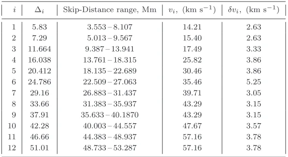
Due to the fact that acoustic waves with the same horizontal phase speed (ω/k) travel the same horizontal distance (∆) the Gaussian phase-speed filter is tuned to select waves with horizontal phase speed (vi) near the ray theory value corresponding to distance ∆i. We define a number of such filters (Fi) corresponding to different

distances (∆i) as follows:

Fi(k, ω; ∆i) = exp[−(ω k −vi)

2

/2δvi2],

where ω is the frequency and k is the horizontal wavenumber in the data power-spectrum. Each filter is applied by pointwise multiplication of the Fourier transform

S(kx, ky, ω)of the observed velocity data.

From the filtered data, we calculate point-to-annulus cross-correlation functions,

C(r_{,∆i, t),for each skip-distance and each position/pixel of our data, where}r_{is the} position vector, ∆i is the distance between two surface bounces and tis time. The

obtained set of cross-correlation functions is then averaged spatially over the quiet Sun to obtain an estimate for the reference cross-correlation function, Cref(∆i, t). This is used to measure one-way travel-time perturbations at each location following Gizon and Birch (2002, 2004, also Jensen and Pijpers, 2003) approach:

τ±= P

i∓f(±ti) ˙C

ref

(ti)[C(ti)−Cref(ti)]

P

if(±ti)[ ˙Cref(ti)]2

, (1)

wheref(t)is a window function designed to pick out the signal from the first bounce (i.e., direct arrival times). Hereτ+ andτ− correspond to wave travelling outwards and inwards from the measurement location respectively. We define the mean travel timesτ(r_,∆)asτ(r_{,∆) = (τ+(}r_{,∆) +τ}−(r,∆))/2.

As a first approximation, perturbations[δτ(r_{,∆)]in these mean travel times are} linearly related to the sound-speed perturbations[δc]in the wave propagation region,

δτ(r_{,∆) =} Z Z

S dr′

Z 0

−d

dzK(r₋r′_{, z; ∆)}δc

2

c2 (r

′

, z), (2)

where S is the area of the region, d is its depth and δτ(r_{,∆) is defined as the} difference between the measured travel time at a given locationr_{on the solar surface} and the average of the travel times in the quiet Sun. The sensitivity kernel for the relative squared sound-speed perturbation is given byK.

For the forward problem we use wave-speed sensitivity kernels estimated using the Rytov approximation by (Jensen and Pijpers, 2003). The Rytov and ray approx-imations give very similar results, with the former being perhaps more reliable for inferring deeper structures (Couvidat, Birch, Kosovichevet al., 2004).

Table 1. Phase speed filter parameters

i ∆i Skip-Distance range, Mm vi, (km s−1) δvi, (km s−1)

1 5.83 3.553 – 8.107 14.21 2.63

2 7.29 5.013 – 9.567 15.40 2.63

3 11.664 9.387 – 13.941 17.49 3.33

4 16.038 13.761 – 18.315 25.82 3.86

5 20.412 18.135 – 22.689 30.46 3.86

6 24.786 22.509 – 27.063 35.46 5.25

7 29.16 26.883 – 31.437 39.71 3.05

8 33.66 31.383 – 35.937 43.29 3.15

9 37.91 35.633 – 40.1870 43.29 3.15

10 42.28 40.003 – 44.557 47.67 3.57

11 46.66 44.383 – 48.937 57.16 3.78

12 51.01 48.733 – 53.287 57.16 3.78

each horizontal wavevectork_{we find the vector}m_{that solves}

min{k(d_−Gm_)k2_2+ǫ(k₎2_kLm_k2_{2}, (3)}

whereLis a regularisation operator. In this work we chose to apply more regularisa-tion at larger depths, where acoustic wave travel times provide less informaregularisa-tion, by setting L = diag(c0,1, . . . , c0,n), where c0,i is the sound speed in the i-th layer

of the reference model. We heavily regularise small horizontal scales (Couvidat, Gizon, Birch et al., 2005) by taking ǫ(k₎2 _{= ǫ}2_{0(1 + (|}k_|/kmax)2₎p _{with p = 200} andǫ2

0= 5×103. We invert for 14 layers in depth located at (0.36, 1.17, 2.11, 3.28,

4.74, 6.41, 8.6, 11.22, 14.28, 17.78, 21.79, 26.31, 31.41, 36.95) Mm.

The errors due to realisation noise are estimated by processing the 24 quiet-Sun datacubes, calculating noise covariance matrix in travel-time measurements (Jensen, 2001; Gizon and Birch, 2004; Couvidat, Gizon, Birch et al., 2005), and then evaluating noise in inversions according to (Jensen, 2001).

2.2. Data

We investigate the active region NOAA 10790 appearing on 13 July 2005. The full disk MDI data with one minute cadence are used. The time series start at 00:00 UT, 10 July 2005, and ends at 23:59 UT 13 July 2005. From this set we extract forty four 512-minute series with the starting times every two hours. Each dataset is then re-mapped and de-rotated onto the heliographic grid using a Postel projection centred at11◦Carrington longitude and11◦latitude (South). The horizontal spread of the data is approximately 380 Mm. We use the Snodgrass rotation rate to remove the differential rotation (Snodgrass and Ulrich, 1990) for each processed datacube.

Figure 2. Sunspot pore emergence. Top panels: the SOHO/MDI intensity (left) and mag-netogram (right) images, taken on 12 July 2005 06:23 UT and 09:35 UT. Bottom panels: the cuts at 11 degrees of latitude through the sound-speed inversion estimated from 512 minute dopplergram timeseries centred on 11 July 2005 08:00 UT (left) and 11 July 2005 10:00 UT (right). The greyscale is inkm s−1_{. Latitude is plotted on the left hand side along they-axis}

and longitude along the x-axis. Depth in Mm is marked on the right hand side of y-axis. Contours correspond to sound-speed perturbation values of0.25and0.3 km s−1_.

3. Results and Discussion

3.1. The Active Region NOAA10790 Surface Emergence and Evolution

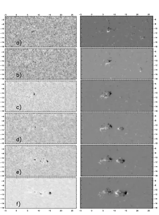
Signs of the increased magnetic activity at the site of the active-region emergence can be first observed on SOHO/MDI magnetogram images taken on 10 July 2005. At this time one can see the two points of flux at around 5◦

–8◦

Carrington longitude. The flux slowly grows with the first pores appearing in the SOHO/MDI continuum images around 11 July 2005 06:30 UT (Figure 1). A number of different pores evolve and disappear at this location until 13 July 2005 06:30 UT, but no sunspots develop. Also around 14:30 UT 13 July 2005, we see a new flux emergence to the east of the first group at around 14◦

longitude,10–12◦

latitude (see Figure 1, panels d) – f)). At this new location, the first sunspot pores appear at about 17:30 UT 13 July 2005, which quickly evolve into the bipolar sunspot group (by 14 July 2005 14:30 UT) before disappearing behind the limb. Also, there is a bipolar region of relatively weak magnetic flux seen appearing at around 20–22◦ longitude on 10 July 2005 and 12 July 2005. No pores were observed at these locations.

3.2. The Subsurface Sound-Speed Inversions

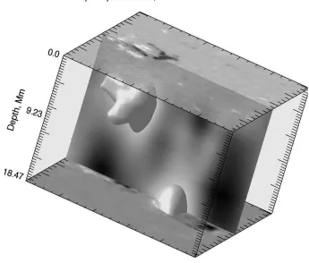
Figure 3. The sound-speed inversion of a 512 minute datacube centred around 13 July 2005 04:00 UT. The top is the surface magnetogram at the start of the time series. The bottom is the surface magnetogram taken around the time of the end of the whole series (14 July 2005 07:59 UT). The vertical panel is the absolute sound-speed perturbation at11◦_{latitude. The}

iso-surface corresponds to a value of 0.32km s−1_.

to see any significant positive sound-speed perturbation in the deeper layers most of the time. This could be due to the fact that the spatial extent of the emerging flux at this location is quite small, six – seven Mm in diameter for each footprint, and the signal cannot be resolved to better than half of the wavelength (Gizon and Birch, 2004). For the power-spectrum produced by the phase-speed filters specified in Table 1, this gives us an estimated resolution of, at best,7.5Mm for waves travelling to

20Mm depths. The averaging kernel at a target depth of 18 Mm, estimated at full width at half-maximum, extends from 8 to 22.5 Mm. This can also be a byproduct of the inversion regularisation, since due to our choice of operator, more regularisation is applied at deeper layers.

As the ratio of gas pressure to magnetic pressure (the plasmaβ) increases rapidly with depth, the sound speed increase due to magnetic field becomes very small,

δc/cof order 0.01 per cent at around 18 Mm below the surface. Using the relations

pe=kTeρe/m,pi =kTiρi/m,pm= B

2

2µ andpe=pi+pm, and assuming that the

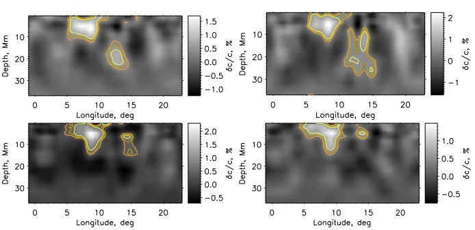
Figure 4. The magnetic flux emergence. The sound-speed inversion as a function of depth and longitude. The cut is made at11◦_{latitude. The inversion is obtained for the 512-minute}

datacubes measured on 13 July 2005. The central times for the Dopplergram time series used to obtain the inversion are (top row): UT 04:00; 06:00; and (bottom row) UT: 08:00; 10:00. Contours drawn for the features located between 4◦_and16◦ _{longitude correspond to}

sound-speed perturbation values of0.5,0.7and1.0per cent.

isc2

A= B

2

µρi, we can evaluate

δc2

c2

e = δT

Te + 2 γβ(1 +

δT Te),

Herepis pressure,Ttemperature,ρdensity,kBoltzman constant,mmean molecular weight, and indices e, i, m stand correspond to external, internal, and magnetic;

β=pi/pm,δc2=c2−c2e,andδT =Ti−Te. Thus, at greater depths the measured perturbation will be dominated by changes in temperature. This makes detecting and following localised perturbations due to emerging magnetic fields difficult.

Notwithstanding the argument above, in our measurements the positive pertur-bation below the surface regions of magnetic activity becomes deeper and better defined as sunspot pores begin to form at the surface, indicating perhaps the increase of magnetic field strength. In the two bottom plots of Figure 2 we can see the region of the increased sound speed extending to depths of around 12 – 15 Mm at around

7◦ longitude that, we believe, is related to the appearance of a sunspot pore seen in SOHO/MDI intensity images. By the time of 13 July 2005 00:00 UT there are several pores observed at this location, and the flux configuration has a clear bi-polar structure (Figure 1c).

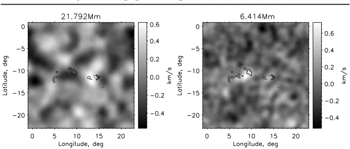
Figure 5. Left: the results of the inversion at 21.77 Mm for the data cube around 13 July 2005 04:00 UT. Right: results of the inversion at 6.41 Mm for the data cube centered around 13 July 2005 08:00 UT. The contours in both plots are lines of±150Gauss from the magnetogram taken around 13 July 2005 17:35 UT.

depth cuts at 21.8 Mm and 6.41 Mm of inversions for series centered on 04:00 UT and 08:00 UT plotted in Figure 5.

One can see the region of increased sound speed at depths of 20 – 25 Mm at about

14◦longitude (see Figure 4, top left, and Figure 5, left). This region can be tracked rising on the next inversion as shown in Figure 4 (top right panel). The regions of increased sound speed can also be seen in the following two inversions (Figure 4, bottom panels) rising to the surface at the location of the second flux group formation. The time of the appearance on the surface (13 July 2005 UT 06:00 – 14:30) corresponds to the first signs of the increased magnetic activity in the surface magnetograms. On the other hand, if the flux, by our assumption represented in the inversions as a region of the increased sound speed, travels from deeper layers to the surface, one should be able to see the traces of this flux presence at deeper layers in the inversions of eight-hour series centered at 08:00 and 10:00, while our inversions show only localised area of sound-speed increase. The averaged resolution kernels estimated for the depths layer around 21.79 Mm at half maximum extend from 8 to 26 Mm.

We are not certain how to interpret this region of negative sound-speed perturba-tion but presumably it is a region of cooler plasma. Under certain condiperturba-tions such a signal could arise from a monolithic flux tube originating in the deeper interior, with internal density exceeding the matter density outside the tube. Alternatively, such an effect can be seen in the scenario described by Kitchatinov and Mazur (2000) in which a temperature instability leads to the formation of an active region due to eddy diffusivity and magnetic tension. If the former explanation is the correct one, then it is tempting to identify such emerging cool flux tubes with the flux tubes postulated by Strous and Zwaan (1999) to explain transient darkenings they observed in continuum intensity.

Thus, we can hypothesize that the sound-speed perturbation seen in Figure 4 is related to the emergence of a hot packet of plasma in the cold plasma column seen in Figure 6. In such circumstances, the absence of a positive perturbation column in the bottom two images of Figure 4 may be due to the dynamic nature of the region considered, wherein the body of increased sound speed preceded and followed by regions of decreased sound speed may cancel each other in our inversion. We note that the inversions of the interior sound speed averaged over eight datacubes obtained on 13 July 2005 (Figure 6, bottom right panel) point to the presence of a decreased sound-speed structure column at the location of the second flux emergence with a positive perturbation directly below the surface. The latter feature can be expected given that these data are for a period after the flux emergence at the surface has become well established. So, if we assume that the region of the increased sound speed corresponds to the emerging magnetic flux and compare the sound-speed per-turbation detected at the depth of 21.7 Mm on 13 July 2005 04:00 and appearing on the surface around 10:00 UT, this can provide an estimate of the speed of emergence at about 1.0 km s−1_{. This estimate is slightly lower than the speed reported by}

(Kosovichev, Duvall, and Scherrer, 2000), but definitely higher than the velocities of a diamagnetic transport in near-surface layers estimated in (Krivodubskij, 2005). This can be an indication of some additional mechanisms affecting the flux emergence.

In our solutions, the errors due to realisation noise are less than 100m s−1: this is estimated by processing the 24 quiet-Sun datacubes and applying the approach described in (Jensen, 2001; Gizon and Birch, 2004; Couvidat, Gizon, Birch et al., 2005).

4. Conclusions

Figure 6. The mean sound-speed perturbation, averaged over all of the processed data, 44 datacubes, (top left) and the mean sound-speed perturbation for the selected dates (averages of 12 datacubes). The greyscale isδc/c in percent. The contours correspond to sound-speed perturbation of 0.1 percent.

We also note that the precise timing of the signature of emergence in the seismic imaging is very limited by the temporal resolution of the sound-speed inversions presented here, since each set is a representative of eight hours of solar oscillations. In view of the dynamo models discussed in Section 1 (Nandy and Choudhuri, 2002, Krivodubskij, 2005), it could be interesting to compare such results for a variety of emerging active regions at different latitudes and stages of the solar cycle.

Acknowledgements We would like to thank an anonymous referee for the valu-able suggestions that have greatly improved this paper. We also acknowledge the sup-port from UK Science and Technology Facilities Council grant number PP/C502914/1.

References

Chang, H.-K., Chou, D.-Y., Sun, M.-T.: 1999, Astrophys. J.,526, 53. Charbonneau, P., MacGregor, K.B.: 1997,Astrophys. J.,486, 502.

Choudhuri, A.R., Schüssler, M., Dikpati, M.: 1995,Astron. Astrophys.,303, 29. Couvidat, S., Birch, A.C., Kosovichev, A.G., Zhao, J.: 2004, Astrophys. J.,607, 554. Couvidat, S., Gizon, L., Birch, A.C., Larsen, R.M., Kosovichev, A.G.: 2005, Astrophys. J.,

158, 217.

Dikpati, M., Charbonneau, P.: 1999,Astrophys. J.,518, 508.

Duvall, T.L. Jr., Jefferies, S.M., Harvey, J.W., Pommerantz, M.A.: 1993, Nature362, 430. Duvall, T.L. Jr., Kosovichev, A. G., Scherrer, P. H., Bogart, R. S., Bush, R. I., de Forest, C.,

Hoeksema, J. T., Schou, J., Saba, J. L. R., Tarbell, T. D., Title, A. M., Wolfson, C. J. and Milford, P. N. : 1997, Solar Phys.170, 63.

Gizon, L., Birch, A.C.: 2002, Astrophys. J.571, 966. Gizon, L., Birch, A.C.: 2004, Astrophys. J.614, 472.

Gizon, L., Birch, A.C.: 2005, Living Reviews in Solar Physics 2, 6–. Jensen, J.: 2001, Ph.D. thesis. Univ. Aarhus.

Jensen, J., Pijpers, F.P.: 2003, Astron. Astrophys.L5, 461.

Jensen, J., Jacobsen, B.H., Christensen-Dalsgaard, J.: 1998, In S. Korzennik & A. Wilson (eds.)Proc. SOHO 6/GONG98 Workshop,SP-418, ESA, Noordwijk, 635.

Kitchatinov, L.L., Mazur, M.V.: 2000,Solar Phys.,191, 325.

Kosovichev, A.G., Duvall, T.L. Jr.: 1997, In F.P. Pijpers, J. Christensen-Dalsgaard, and C.S. Rosenthal (eds) SCORe’96 : Solar Convection and Oscillations and their Relationship, ASSL 225, Kluwer Academic, 241.

Kosovichev, A.G., Duvall, T.L. Jr., Scherrer, P.H.: 2000, Sol.Phys., 192, 159. Krivodubskij, V.N.: 2005, Astron. Nachr.,326, 61.

Nandy, D., Choudhuri, A.R.: 2002,Sci., 296, 1671.

Parker, E.N.: 1979,Cosmical Magnetic Fields, Clarendon Press, Oxford. Parker, E.N.: 1993,Astrophys. J.,351, 309.