The turbulence velocity gradient tensor formed additively by normal and non-normal tensors

This is a repository copy of The turbulence velocity gradient tensor formed additively by normal and non-normal tensors.

White Rose Research Online URL for this paper: http://eprints.whiterose.ac.uk/108949/

Article:

Keylock, C.J. orcid.org/0000-0002-9517-9896 The turbulence velocity gradient tensor formed additively by normal and non-normal tensors. (Unpublished)

eprints@whiterose.ac.uk https://eprints.whiterose.ac.uk/

Reuse

Unless indicated otherwise, fulltext items are protected by copyright with all rights reserved. The copyright exception in section 29 of the Copyright, Designs and Patents Act 1988 allows the making of a single copy solely for the purpose of non-commercial research or private study within the limits of fair dealing. The publisher or other rights-holder may allow further reproduction and re-use of this version - refer to the White Rose Research Online record for this item. Where records identify the publisher as the copyright holder, users can verify any specific terms of use on the publisher’s website.

Takedown

If you consider content in White Rose Research Online to be in breach of UK law, please notify us by

arXiv:1608.01261v1 [physics.flu-dyn] 3 Aug 2016

The turbulence velocity gradient tensor formed additively by

normal and non-normal tensors

C. J. Keylock

Sheffield Fluid Mechanics Group and Department of Civil and Structural Engineering,

University of Sheffield, Mappin Street, Sheffield, U.K., S1 3JD ∗

(Dated: August 4, 2016)

I. INTRODUCTION

An enhanced understanding of how a turbulent flow dissipates energy is crucial for linking

the topological view of turbulence to the statistical considerations of dissipation and, hence,

developing the next generation of numerical closure schemes for modeling high Reynolds

number flows in industry and the environment. This is an old problem with pioneering work

undertaken by G. I. Taylor in the 1930s [1], and Betchov in the 1950s [2], and significant

progress having been made since the advent of high Reynolds number computations [3–5].

The Navier-Stokes equations can be written in terms of the velocity-gradient tensor

Aij =

_∂u

1/∂x1 ∂u1/∂x2 ∂u1/∂x3

∂u2/∂x1 ∂u2/∂x2 ∂u2/∂x3

∂u3/∂x1 ∂u3/∂x2 ∂u3/∂x3

, (1)

and a topological classification of the flow can be developed using the characteristic equation

forA[6]: λ3_{+ Pλ}2_{+ Qλ+ R = 0 , where P =−}P

λi = 0 in an incompressible flow because

of the divergence-free constraint, and the λi are the eigenvalues of A. The term Q may be

interpreted as the excess of total enstrophy to total strain and has become popular as a means

to visualize coherent structures [7, 8]. That is, if A is decomposed into symmetric strain

rate and skew-symmetric rotation rate components as Aij = Sij + Ωij, Q = −1₂tr(A2) =

1

2 Ω

2 _{− S}2

, where Ω2 _{is the total enstrophy and S}2 _{is the total strain. Transforming}

rotation into the vorticity,ω =ǫ_ijkΩ, whereǫ_ijkis the Levi-Civita symbol, leads to transport

equations for these terms:

1 2

DS2

Dt =−SijSjkSki−

1

4ωiωjSij

−Sij

∂2_p

∂xi∂xj

+νSij∇2Sij

1 2

Dω2

Dt =ωiωjSij +νωi∇

2_ω

i, (2)

The deviatoric part of the pressure Hessian, ₋Sij ∂

2

p

∂xi∂xj, contains important information on

the non-local properties of turbulence [9–11]. However, in the mean, its contribution is

zero [12], meaning that a popular approach to analyzing the evolution of total strain and

enstrophy is the reduced Euler framework [13]. This means that the key terms are the

strain rate production, ₋SijSjkSki and enstrophy production, ωiωjSij. These appear in the

equation for R:

R =₋detλi =

1

3 −SijSjkSki− 3

4ωiωjSij

and the discriminant function in Q₋R space that separates regions with a conjugate pair

of eigenvalues (that act as saddles or nodes) to those where all λi ∈ ℜ (that act as foci) is

given by D = Q3+ (27/4)R2 [14]. While studies of the dynamics of the velocity gradient tensor typically analyze the flow in a Q₋ R space [6, 15] it has been argued that this

space needs to be expanded into three dimensions because the Lagrangian dynamics in a

Q₋SijSjkSki−ωiωjSij space reveals novel and complementary properties on the Q−ωiωjSij

plane [16].

The intention of this paper is to propose a contrasting mathematical starting point for

an additive decomposition of A based on the notion of matrix/tensor normality, and to

demonstrate the fluid mechanical relevance of such an approach. This includes some new

insights into results for the paradigmatic case of homogeneous, isotropic turbulence.

II. TENSOR NORMALITY

If A is normal, then

AAH =AHA, (4)

where H is the conjugate transpose. IfAAH ₆=AHAthen there are some ‘residual’

dynam-ics that exist independent of the eigenvalue representation of A. This may be made explicit

by considering the Schur decomposition of A:

UTUH =A

T=Λ+N

UΛUH =B

UNUH =C, (5)

where U is unitary and the Schur matrix, T, may be decomposed into a diagonal matrix

of eigenvalues, diag(Λ) = λ1, . . . , λ3 and an upper triangular matrix, N that characterizes

the non-normality of A [17]. We use a complex Schur transform to ensure T is triangular,

rather than the quasi-triangular real form. While this has the disadvantage that B and C

are potentially complex, computational uncertainties in moving from complex to real forms

are obviated. In practice, we work with the strain rate and rotation rate tensors derived

from B and C, i.e. SB = 1₂ B+BH

; ΩB = 1₂ B−BH

, which side-steps this issue. As

An alternative definition of non-normality to (4) is _||A_||2_{F − ||}Λ_||2_F = _||N_||2_F, meaning that the Frobenius norm, _||. . ._||F =

q

tr(AAH) is a logical choice for this problem. It

follows immediately that_||A_||2_F =_||B_||F2 +_||C_||2_F,_||SA||2_F =||SB||2_F+||SC||2_F, and||ΩA||2_F =

||ΩB||2_F||+||ΩC||2_F, while Pλ(

C)

i = 0 means that ||SC||_F =||ΩC||_F. As a consequence, we

may write that

||A_||2_F =_||SB||2_F + 2||SC||2_F +||ΩB||2_F. (6)

This leads us to two indices characterizing the ratio of the norms for the straining parts of

B and C, and the ratio of the straining and rotational norms ofB, respectively:

κ1 = ||

SB||2_F −2||SC||2_F

||SB||2_F + 2||SC||2_F

κ2 = ||

ΩB||2_F − ||SB||2_F

||ΩB||2_F +||SB||2_F

. (7)

To these, we add a third measure that examines the straining properties of B. That is, we

apply the Lund and Rogers normalization [18] to B rather than its standard application to

A:

κ3 ≡e(

B)

LR =

3√6R(SB)

−2Q(SB)

32

. (8)

III. RESULTS

This study makes use of the Johns Hopkins numerical simulation of HIT at a Taylor

Reynolds number of 433 [19], which has become a popular resource for studying flow

topolo-gies [20, 21]. Here we interrogated a 10243 _{volume of the database at one point in time, a}

strategy that has been adopted previously [11]. We first show some of the physics that can

be uncovered with our approach, before exploring some of the properties of the κ planes.

Our analysis is conditioned on alignments of the strain eigenvectors, as well as locations in

Q₋R space.

A. Properties of the second eigenvector of the strain tensor

An important property of homogeneous, isotropic turbulence (HIT) is the tendency for

the Lund and Rogers normalization of A to give values close to +1 as a consequence of

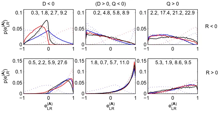
−1 0 1 0 0.05 0.1 p(e LR (A ) )

D < 0

−10 0 1

0.05 0.1

(D > 0, Q < 0)

−1 0 1

0 0.05 0.1

Q > 0

−1 0 1

0 0.05 0.1 0.15 e LR (A) p(e LR (A ) )

−10 0 1

0.05 0.1 0.15 e LR (A)

−1 0 1

0 0.05 0.1 0.15 e LR (A)

R < 0

R > 0 0.3, 1.8, 2.7, 9.2 0.2, 4.8, 5.8, 8.9

1.8, 0.7, 5.7, 11.0

2.2, 17.4, 21.2, 22.9

5.3, 1.9, 8.6, 9.5 0.5, 2.2, 5.9, 27.6

FIG. 1. Histograms of the Lund and Rogers normalization for the second eigenvalue of the strain tensor of A as a function of Q, D, R, and the dominant alignment between strain eigenvectors given by max

cos(e(_iA),e(_iB,C))

>0.9397, wherei= 1 are in blue,i= 2 in black, andi= 3 in red. Alignments between e(_iA) and e(_iB) are displayed as solid lines, and e(_iA) and e(_iC) as dotted lines. Four numbers are quoted in each panel. From left to right these are the percentage occurrence in a given panel for

e(₁A),e(₁C), (blue, dotted lines),

e(₃A),e(₃C) (red, dotted lines), P

e(_iA),e(_iC)

(all dotted lines), and all the displayed results.

Schur decomposition to partition the results by strain eigenvector alignments as shown in

Fig. 1. The six dominant strain eigenvector alignments shown in each panel account for

89% of the total data (i.e. the sum of the right-hand numbers in each panel). This was

because in 5% of cases, there was no observed alignment where cos(e(_iA),e_i(B,C)) > 0.9397 (i.e. _±20 degrees from perfect alignment), and in 6% of cases, the strongest alignment was

not between strain eigenvectors of the same rank order, i.e. max

cos(e(_iA),e(_jB,C))

>0.9397,

but i₆=j.

When Q>0, dominant alignments are between SA and SC (93% of cases for R<0 and

91% for R> 0), and the proportion of tensors where this is true for R< 0 always exceeds

that for R >0 (65% compared to 52% when D>0, Q<0, and 29% compared to 21% for

D <0). Furthermore, a dominant alignment between

e(₁A),e(₁C)

always detracts from the

+1 alignment, while

0 0.1

negative S_ijS_jkS_ki

0 0.1 0 0.1 0 0.1 probability 0 0.1 −2 0 2 4 0 0.1

log₁₀(|S_ijS_jkS_ki|)

positive S_ijS_jkS_ki

−2 0 2 4

log₁₀(|S_ijS_jkS_ki|)

0 0.05 0.1

negative ω_iω_jS_ij

0 0.05 0.1 0 0.05 0.1 0 0.05 0.1 0 0.05 0.1 −2 0 2 4 0 0.05 0.1

log₁₀(|ω_iω_jS_ij|)

positive ω_iω_jS_ij

−2 0 2 4

log₁₀(|ω_iω_jS_ij|)

[e₁(A),e₁(B)]

[e 1 (A)_,e

1 (C)_]

[e₃(A),e₃(C)]

R < 0 R < 0

R > 0 R > 0

[e 2 (A)_,e 2 (C)_] [e 3 (A)_,e 3 (B)_] [e 2 (A)_,e 2 (B)_]

FIG. 2. Histograms of selected distribution functions, as discussed in the text, for strain production, SijSjkSki, and enstrophy production ωiωjSij. The abscissa is on a log-scale and positive and negative contributions have been separated. In each panel, the dotted line is for the D<0 case, the solid line is the (D>0,Q<0) case, and the thick solid line is the Q>0 case.

contrast to the alignments betweenSA and SC, those betweenSA andSB, generally exhibit

a similar behavior to each other. Exceptions include the D < 0, R < 0 region (10% of all

cases), where

e(₃A),e₃(B)alignments detract from thee(_LRA) _∼+1 relation to a greater extent, and where

e(₁A),e(₁B)

(the dominant alignment here, representing 4.6% of all cases) gives a

clear preference for a plane shear configuration of the velocity gradient tensor, e(_LRA) _∼0. It is clear that when the flow is close to the Vieillefosse tail (R >0 and Q <0), we find

e(_LRA) _∼1, with the exception of

e(₁A),e(₁C) (although this only occurs for 0.5 + 1.8 = 2.3% tensors). Because this region accounts for 38.6% of the data, strong signs of axisymetric

ex-tension are required elsewhere in Q₋R space for this state to be so prevalent. Consequently,

the contribution by

e(₃A),e(₃C) when R < 0 (24% of all the cases) is crucial, particularly when Q > 0 (17.4%). Indeed, if it were not for this alignment state, the e(_LRA) = 1 pattern would really be a Vieillefosse tail phenomenon, only. The dominance of the

e(₃A),e(₃C)

alignment in this region also explains the large positive enstrophy production (the only part

of the Q₋R space where this occurs so strongly[12]) and weak strain production found here.

This is shown in the first row of Fig. 2.

e₃(A),e₃(C) when (R < 0,Q > 0) , the second most dominant occurence of all is when (Q > 0, R > 0), and involves

e(₁A),e(₁C). These data are shown in the third row of Fig. 2 and show very different behavior to the other R > 0 cases shown, with very strong

negative enstrophy production driving the response, rather than positive strain production.

The other R > 0 cases highlighted include those involving second eigenvector alignments,

which emerge as important near the Vieillefosse tail, with

e(₂A),e(₂B)

more important as

one approaches from below (D<0), and

e(₂A),e(₂C) from above (D>0).

From the perspective of Taylor’s result that _hωiωjSiji >0 [1], our results clearly permit

the alignments that act counter to this average behavior to be discerned, and the case where

this arises irrespective of position on the Q-axis when R >0 is

e(₁A),e(₁C). The fifth and fourth rows also show that this situation occurs where

e(₃A),e(₃B)

dominates for D>0, and

e₂(A),e₂(B,C) for Q>0.

The second most important alignment when R<0, is

e(₁A),e(₁B)

, which grows from 4%

of cases for Q>0, through 22% for (D >0,Q<0), to 46% for D<0. The first two rows

of Fig. 2 show an important difference with R < 0 arising because of positive enstrophy

production in both cases, but ₋SijSjkSki counteracting positive enstrophy production in

the first row, and negative strain production acting with positive enstrophy production in

the second row. Indeed, this is a consistent property: if the dominant alignment is between

SA and SB there is a ‘consistent’ behavior for predicting the sign of R from the production

terms. In contrast more refined analysis of the balance of these terms is needed when the

dominant alignments are between SA and SC. Hence, while the dynamical significance of

separating R into its constituents has already been shown [16], a new rationale for this may

be offered here: When dominant strain alignments are betweenSAandSCthe sign of R does

not determine the nature of strain and enstrophy production in any simple way. Because the

eigenvalues forAandBare identical, their behavior in Q₋R is also identical. Consequently,

disaggregating into the constituent terms is essential for revealing the contribution of C to

the fluid mechanics of trajectories within the space of the reduced Euler approximation.

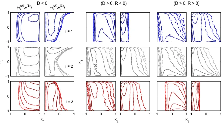
IV. PROPERTIES OF THE κ DECOMPOSITION

Mathematical constraints on the values forκ2 and κ3 in (7) and (8) simplify our analysis

−1 0 1 −1

0 1

−1 0 1

κ3

−1 0 1 −1 0 1

−1 0 1 −1 0 1

κ2

−1 0 1 −1 0 1

κ₁ κ₁ κ₁

(e

i (A)

,e

i (B)

) (e

i (A)

,e

i (C)

)

D < 0 (D > 0, R < 0) (D > 0, R > 0)

i = 2 i = 1

i = 3

FIG. 3. Contour plots of the joint probability of κ1 −κ3 for D < 0 and κ1 −κ2 for D > 0 as a

function of the strain alignments also used in Fig. 1. These latter results are sub-divided by the sign of R. Each two-column set of results shows the strain alignments for (e(_iA),e(_iB)) (left-hand column) and (e(_iA),e(_iC)) (right-hand column). The blue, gray, and red contours are for i = 1, i= 2, andi= 3, respectively. The contour lines are distributed on a logarithmic scale from 10−5 to 10−2 _{in half-integer intervals of the power of ten.}

• Aκ1−κ3 plane if D<0 (withκ3 =±1 for D>0;κ3 =−1 if R<0,κ3 = 1 if R>0);

and,

• A κ1−κ2 plane if D >0 (with D<0 values at κ2 =−1).

The κ2 term has the property that 0 < κ2 ≤ 1 corresponds to Q > 0 and −1 < κ2 < 0

corresponds to D > 0 and Q < 0. That is, the discriminant function in Q₋R space is

recast here as the relative magnitudes of the Frobenius norms for the symmetric and

skew-symmetric parts of B. The corresponding constraint for κ3 is that 0 < κ3 ≤ 1 equates to

R>0 and₋1< κ3 <0 to R<0.

As the dominant alignments are between [e(_iA),e_i(B) when D < 0 (Fig.1), we find κ1

is typically positive for these cases in the κ1 −κ3 plane. Given that κ3 is the Lund and

Rogers normalization ofSB, this positive tendency is indicative of a dominant axisymmetric,

When D > 0 the behavior of [e(_iA),e(_iB) depends on both the sign of R and that of Q: first eigenvector alignment when R < 0 (third column) and third when R > 0 (fifth

column) gives κ1 > 0. Otherwise, Q > 0 (upper half of the κ1 −κ2 planes) gives a more

negative response, which dominates the distribution functions when R < 0. In contrast,

when [e(_iA),e_i(C) alignments are dominant, κ1 is strongly negative. The exception to this

are the [e(₂A),e(₂C)

cases in the vicinity of the Vieillefosse tail (upper half of the panel in the

middle row, second column; lower half of the of the panel in the middle row, sixth column).

This highlights a property of straining in this region that differs from other cases and is not

discernible in the production terms shown in Fig. 2.

V. CONCLUSION

While consideration of turbulence in a Fourier shell representation views dissipation as a

small-scale phenomenon, when studying spatial fields at small-scales (near to Kolmogorov

scales), where velocity derivatives dominate, all locations are ‘small’. Hence, focus moves

toward the locations where particular phenomena occur, leading to the increasing focus on

the topological approach [5, 6, 22] to understand processes such as dissipation [23, 24]. Here

we have proposed a new representation of the topological space for these phenomena based

on a decomposition of the velocity gradient tensor into normal and non-normal components.

Because the eigenvalues of the former are equal to those of the velocity gradient tensor, their

Q₋R representations are equivalent. Hence, explicit consideration of non-normality provides

a richer representation, complementing the pre-existing suggestion to separate enstrophy

production and strain production terms [16].

Enhanced closure models for engineering models of turbulent fluid flow are likely to be

based on knowledge of Lagrangian walks around such topology spaces [25, 26]. Ourκ1−κ2,3

planes provide a new way to formulate such models. An extension of the current work is

therefore an examination of the Lagrangian dynamics inκ1−κ2,3 space, perhaps conditioned

on the strain alignments that have been shown to be of dynamical importance here. Another

area to explore would be the extension of the reduced Euler system to incorporate pressure

alternative means to describe spatially intermittent dissipation in a modeling context [27].

[1] G. I. Taylor, Proc. R. Soc. Lond. A 164, 15 (1938). [2] R. Betchov, J. Fluid Mech. 1, 497 (1956).

[3] R. M. Kerr, J. Fluid Mech.153, 31 (1985).

[4] W. T. Ashurst, A. R. Kerstein, R. A. Kerr, and C. H. Gibson, Phys. Fluids 30, 2343 (1987). [5] C. Meneveau, Ann. Rev. Fluid Mech. 43, 219 (2011).

[6] M. S. Chong, A. E. Perry, and B. J. Cantwell, Phys. Fluids A 2, 765 (1990).

[7] J. C. R. Hunt, A. A. Wray, and P. Moin,Eddies, stream, and convergence zones in turbulent flows, Tech. Rep. CTR-S88 (Center for Turbulence Research, 1988).

[8] Y. Dubief and F. Delaycre, J. Turbul.1 (2000).

[9] K. Ohkitani and S. Kishiba, Phys. Fluids7, 411 (1995).

[10] L. Chevillard, C. Meneveau, L. Biferale, and F. Toschi, Phys. Fluids20, 101504 (2008). [11] M. Wilczek and C. Meneveau, J. Fluid Mech.756, 191 (2014).

[12] A. Tsinober, inTurbulence Structure and Vortex Dynamics, edited by J. C. R. Hunt and J. C. Vassilicos (Cambridge University Press, 2001) pp. 164–191.

[13] B. J. Cantwell, Phys. Fluids A4, 782 (1992).

[14] A. E. Perry and M. S. Chong, Annu. Rev. Fluid Mech. 19, 125 (1987). [15] A. Tsinober, L. Shtilman, and H. Vaisburd, Fluid Dyn. Res.21, 477 (1997). [16] B. L¨uthi, M. Holzner, and A. Tsinober, J. Fluid Mech. 641, 497 (2009).

[17] G. H. Golub and C. F. van Loan, Matrix Computations, 4th ed. (Johns Hopkins University Press, 2013).

[18] T. S. Lund and M. M. Rogers, Phys. Fluids6, 1838 (1994).

[19] Y. Li, E. Perlman, M. Wan, Y. Yang, R. Burns, C. Meneveau, S. Chen, A. Szalay, and G. Eyink, J. Turbulence 9 (2008).

[20] M. Wan, Z. Xiao, C. Meneveau, G. L. Eyink, and S. Chen, Phys. Fluids22, 1 (2010). [21] J. M. Lawson and J. R. Dawson, J. Fluid Mech. 780, 60 (2015).

[22] Y. Zhou, K. Nagata, Y. Sakai, H. Suzuki, Y. Ito, O. Terashima, and T. Hayase, Phys. Fluids 26, 045102 (2014).

[24] S. Goto and J. C. Vassilicos, Phys. Fluids 21, 035104 (2009). [25] J. Mart´ın, C. Dopazo, and L. Vali˜no, Phys. Fluids10, 2012 (1998).