Estimation of Precipitable Water Using Numerical Prediction Data

Article

Estimation of Precipitable Water Using Numerical

Prediction Data

Shin

Akatsuka

_{, Junichi}

_Susaki

_{, and Masataka}

_Takagi

1 School of Systems Engineering, Kochi University of Technology, 185, Miyanokuchi, Tosayamada, Kami,

Kochi 782-8502, Japan

2 Department of Civil and Earth Resources Engineering, Graduate School of Engineering, Kyoto

University, Kyoto-daigaku katsura, Nishi-kyo ku, Kyoto 615-8540, Japan

E-mail: a_{[email protected] (Corresponding author),} b_{[email protected],} c_{[email protected]}

Abstract. Precipitable water (PW) is an important variable in the climate system.

Interferometric synthetic aperture radar (InSAR) is a powerful remote sensing technique for measuring the topography and deformation of the Earth’s surface. However, variations in atmospheric water vapor content affect the accuracy of InSAR measurements. Therefore, it is important to understand the distribution of PW to mitigate atmospheric effects on remote sensing data. Herein, we estimated the PW distribution with high spatial resolution using numerical prediction data and digital elevation model (DEM) data from the Kanto region of Japan. We estimated the PW distribution at a resolution of 90 m from mesoscale model grid point value data while accounting for the difference in surface elevation within pixels using DEM data with a resolution of 90 m. The PW distribution at 90-m resolution could be estimated using the proposed method with good accuracy (root-mean-square difference within 4.0 mm) throughout the year. The proposed method provides high-resolution information on atmospheric water vapor content and its variation at 3-h intervals. This method is expected to be applicable in climate research and for the atmospheric correction of remote sensing data, which can improve the accuracy of remote sensing measurements.

Keywords: Atmospheric water vapor, climate change, remote sensing, DEM.

ENGINEERING JOURNAL Volume 22 Issue 3

Received 12 January 2018 Accepted 13 February 2018 Published 28 June 2018

1.

Introduction

Precipitable water (PW) is the total atmospheric water vapor contained in a vertical column from the Earth’s surface to the top of the atmosphere. PW is an important variable in the climate system, hydrological systems, and terrestrial ecosystems. For example, atmospheric water vapor is one of the greenhouse gases that lead to global warming. Water vapor influences the partitioning of incoming solar radiation into latent and sensible heat fluxes through its effects on stomatal conductance and evapotranspiration [1]. In turn, this process feeds back into the Earth’s energy and water budgets [1]. According to model simulations, increased atmospheric water vapor content generates the single largest positive feedback on surface temperature and is a major factor in precipitation augmentation at middle and high latitudes [2]. Therefore, it is necessary to monitor changes in atmospheric water vapor content to validate the large feedback caused by atmospheric water vapor in climate models and to detect global warming [2].

Atmospheric water vapor content is also critical for atmospheric correction, which is the most important step in the pre-processing of remote sensing data. Interferometric synthetic aperture radar (InSAR) is a powerful remote sensing technique for measuring the topography and deformation of the Earth’s surface. These measurements are based on the phase differences in the signal backscattered by the land surface at two acquisition dates after correcting for orbital contributions [3]. However, variations in atmospheric water vapor content affect the accuracy of InSAR measurements. The dominant source of error in InSAR measurements is differential propagation path delay caused by the large spatial and temporal variability in atmospheric water vapor content [4, 5]. This variability is easily misinterpreted as a surface deformation, thus limiting the accuracy of InSAR measurements [5]. Therefore, high-resolution information on atmospheric water vapor content and its variation with time are crucial to mitigate the effects of wet tropospheric path delay variations on InSAR interferograms [6].

PW is mainly measured using radiosondes over land; however, these instruments are limited in their ability to make continuous measurements of PW with good spatial resolution [7]. Although PW can also be measured by ground-based global positioning system (GPS) data [8-10], this method results in poor temporal and/or spatial resolution [11]. Compared with traditionally used ground-based meteorological observations, space-based monitoring provides high spatial resolution over large areas of the Earth’s surface and is particularly useful in isolated locations where meteorological observation stations are rare [12]. Space-based monitoring is an effective way of measuring the global distribution of water vapor with a spatial resolution much closer to the resolution of SAR images compared with the station spacing of GPS networks [13]. However, space-based monitoring is sensitive to the presence of clouds in the field of view [13], and it is not always available at the time corresponding to SAR data acquisition [3]. Current numerical weather prediction (NWP) models can provide the high spatial resolution necessary to reproduce realistic distributions of water vapor. Therefore, the water vapor fields produced by NWP are able to eliminate some of the problems described above [11].

Consistent time series of PW vapor are important in meteorology and climate research [14] and in remote sensing. The purpose of this study is to estimate the PW distribution at high spatial resolution using NWP and digital elevation model (DEM) data from the Kanto region of Japan. Although the spatial resolution of NWP data is 5 km at the surface and 10 km at each barometric surface, we estimated the PW distribution with a resolution of 90 m by accounting for the differences in surface elevation within pixels using DEM data with a resolution of 90 m.

2.

Data Description

Table 1. Description of MSM GPV data.

Variable Level Spatial resolution (km)

Temporal resolution (h)

Air temperature (K) Surface 5 1

Relative humidity (%) Surface 5 1

Surface pressure (hPa) Surface 5 1

Sea-level pressure (hPa) Surface 5 1

Air temperature (K) 16 pressure levels* 10 3

Relative humidity (%) 12 pressure levels** 10 3

* 16 pressure levels: 1000, 975, 950, 925, 900, 850, 800, 700, 600, 500, 400, 300, 250, 200, 150, 100 hPa.

** 12 pressure levels: 1000, 975, 950, 925, 900, 850, 800, 700, 600, 500, 400, 300 hPa.

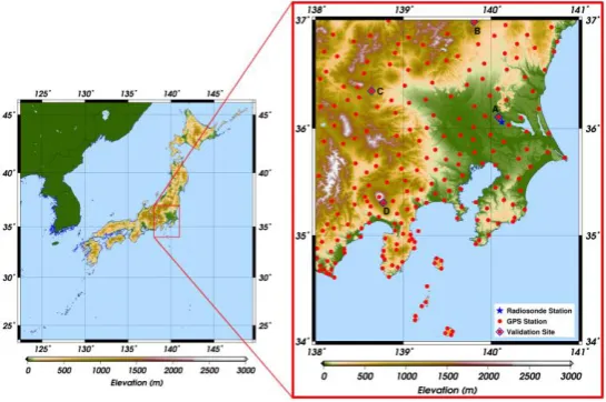
We used Advanced Spaceborne Thermal Emission and Reflection Radiometer (ASTER) Global Digital Elevation Model (GDEM) data as the DEM data. These data are generated using stereo-pair images collected by the ASTER instrument onboard Terra [16]. The original spatial resolution of ASTER GDEM data is approximately 30 m (1 arcsecond); in this study, the data were resampled to a spatial resolution of 90 m in order to reduce processing time. ASTER GDEM is shown in Fig. 1 as the base map.

The PW values estimated from radiosonde observation and ground-based GPS data were used to validate the PW estimated from MSM GPV data. Radiosonde observation was conducted twice a day at 0000 UTC and 1200 UTC at Tateno in the Kanto region of Japan (Fig. 1). The PW derived from radiosonde observation data at Tateno in 2014 was downloaded from the “Atmospheric Soundings” website of the University of Wyoming [17]. The PW at the GPS stations can be estimated from the travel-time delays of global GPS signals between satellites and ground-based receivers if the temperature and pressure at the GPS stations are known [18]. According to previous studies [19, 20], we calculated the GPS-derived PW at 3-h intervals in 2014 from the atmospheric delay data provided by the Geospatial Information Authority of Japan and the temperature and pressure at each GPS station interpolated from the observed values of JMA’s Automated Metrological Data Acquisition Systems.

3.

PW Estimation from Numerical Prediction Data

3.1. PW Calculation

The integrated water vapor content was derived using the following formula [21]:









0,1 0 1 1,2 1 2

100

PW q P P q P P

g  

 _     _, (1)

Where PW is precipitable water (mm), qi,i+1 is the mean specific humidity (kg kg−1) between a layer bounded

by pressures Pi and Pi+1 (hPa), and g is acceleration due to gravity.

3.2. PW Estimation from MSM GPV and DEM Data

If we can estimate the specific humidity at each barometric surface of MSM GPV data, PW can be calculated using Eq. (1).

The specific humidity at pressure level Pn can be calculated using Eq. (2):



0.622



0.378

n

n P

q

P e





where qn is the specific humidity (kg kg−1) at pressure level Pn and ePn is the water vapor pressure (hPa) at

MSM GPV pressure level Pn.

The water vapor pressure at pressure level Pn can be calculated using Eq. (3):

,

100

n

n n

P

P P sat

RH

e





_



_



e





where ePn is the water vapor pressure (hPa) at pressure level Pn, RHPn is the relative humidity (%) at pressure

level Pn, and en,sat is the saturation water vapor pressure (hPa) at pressure level Pn.

The saturation water vapor pressure at pressure level Pn can be calculated using Eq. (4) [22]:









,

6.1094 exp 17.625

243.04

n n n

P sat P P

e





T



T

where ePn,sat is the saturation water vapor pressure (hPa) at pressure level Pn and TPn is the air temperature

(°C) at pressure level Pn.

MSM GPV data include the relative humidity and air temperature at 12 pressure levels (1000–300 hPa); thus, we can calculate PW between the surface and the 300 hPa pressure level using Eqs. (1)–(4). Because the spatial resolution of MSM GPV data is 5 km at the surface and 10 km at each barometric surface level, we estimated the PW distribution at a resolution of 5 km from MSM GPV data using Eq. (5):













1000 1000 975 400 300

1000 1000 975 400 300

100

2

2

2

S

S

q

q

q

q

q

q

IWV

P

P

P

P

P

P

g













_







 



_





where IWV is the integrated water vapor content between the surface and the 300 hPa pressure level (mm),

PS is the surface pressure (hPa), and qS is the specific humidity (kg kg−1) at the surface level. In this study,

the IWV between the surface and the 300 hPa pressure level is taken as PW.

Here, we focus only on a grid of MSM GPV data (Gmn) and a DEM pixel (Dij) within Gmn. The PW of

Dij can be calculated from the specific humidity and surface pressure of Dij, which can be estimated from

both the MSM GPV and DEM data.

Assuming that air is an ideal gas and that the temperature lapse rate is 6.5 K km−1_{, the elevation of Gmn}

(HGmn) can be calculated using the following relation [23, 24]:

1 5.257 ,

273.15

1

0.0065

G SL G

G G

T

P

H

P



_

_





_

_







_



_

















, (6)

where TGmn, PGmn, and PSL,Gmn are the surface air temperature (°C), surface pressure (hPa), and sea-level

pressure of Gmn (hPa), respectively.

The surface pressure of Dij (PDij), whose elevation is hDij (m), can be expressed using TGmn, PSL,Gmn, and hDij as

[23] 5.257 , ,

0.0065

1

273.15

D SL G

SL G

h

P

P

T







 



_



_







where TSL,Gmn is the sea-level air temperature (°C), which can be derived from Eq. (8) as

, mn mn

0.0065

SL G G G

T



T



H

The specific humidity of Dij (qDij) can be calculated from Eq. (9) as [25]





ij ij ij D D D q P e 

 . (9)

From Eqs. (3) and (4), the saturation water vapor pressure of Dij (eDij) can be calculated from Eq. (10)

as









6.1094 exp 17.625 243.04

100

ij

ij ij ij

D

D D D

RH

e _ _  T T

  , (10)

where TDij is the sea-level air temperature (°C), which can be derived from Eq. (11):

T_D

ij =TSL,Gmn-0.0065hDij. (11)

Finally, if PDij > 1000 hPa, we assume that RHDij = RHGmn, and the specific humidity of Dij (qDij) can

then be estimated using Eqs. (7)–(11). If PDij≦ 1000 hPa, we assume that qDij = qPn,Gmn; qPn,Gmn is the specific

humidity of Gmn at pressure level Pn, which is the nearest barometric surface of PDij.

For PDij > 1000 hPa, the PW of Dij can be estimated by













1000 _{1000 975 400 300}

1000 1000 975 400 300

100

2 2 2

ij

ij ij

D

D D

q q _{q q q q}

PW P P P P P P

g



   

 _       _

  (12)













1 1 2

, 400 300

1 1 2 400 300

100

2

2

2

n mn

ij ij

P G P P P

D D

q

q

q

q

q

q

PW

P

P

P P

P

P

g













_







 



_





(P2 < P1 < PDij≦ 1000).

3.3. Validation of Estimated PW

According to the procedure explained in Section 3.2, the 90-m-resolution PW was estimated at 3-h intervals using 2014 MSM GPV and ASTER GDEM data. From this point forward, we refer to this estimated PW as MSM-refined PW. To validate MSM-refined PW, we extracted the MSM-refined PW values at the pixels where Tateno and TSUKUBA3 are located, and compared them with radiosonde PW at Tateno and GPS PW at TSUKUBA3. TSUKUBA3 is the nearest GPS station to Tateno, and the distance between TSUKUBA3 and Tateno is approximately 6 km. The annual biases and root-mean-square (RMS) differences between MSM-refined PW and radiosonde PW at Tateno in 2014 were calculated at 0000 UTC and 1200 UTC. The biases at 0000 UTC and 1200 UTC in 2014 were −0.3 and −0.5 mm, respectively, and the RMS differences were 3.0 and 3.3 mm, respectively. The left column of Fig. 2 shows the scatter plots of MSM-refined PW and radiosonde PW values at Tateno. The center column of Fig. 2 shows the scatter plots of MSM-refined PW and GPS PW at TSUKUBA3; the RMS differences at 0000 UTC and 1200 UTC were 1.7 and 1.4 mm, respectively. The right column of Fig. 2 shows the scatter plot between GPS PW at TSUKUBA3 and radiosonde PW at Tateno; the RMS differences at 0000 UTC and 1200 UTC were 3.0 and 3.4 mm, respectively. As shown in Fig. 2, although some large differences were observed, MSM-refined PW generally showed good agreement with GPS- and radiosonde-based PW throughout the year. Because no large differences were observed between MSM-refined PW and GPS PW, the large discrepancies between MSM-refined PW and radiosonde PW are likely attributed to error in the radiosonde measurements.

Fig. 2. Scatter plots among MSM-refined PW, GPS PW, and radiosonde PW in 2014 (upper row: 0000 UTC; lower row: 1200 UTC): left column, scatter plots between MSM-refined PW and radiosonde PW at Tateno; center column, scatter plots between MSM-refined PW and GPS PW at TSUKUBA3, which is the nearest GPS station to Tateno; and right column, scatter plots between GPS PW at TSUKUBA3 and radiosonde PW at Tateno.

4.

Elevation Correction

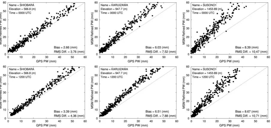
mountainous regions because of the large differences in altitude between the real topography and its representation in the weather forecasting model. Figure 3 shows scatter plots between MSM-refined PW and GPS PW at validation sites (SHIOBARA, KARUIZAWA, and SUSONO1 at elevations of 566.8, 947.7, and 1453.9 m, respectively; Fig. 1) in 2014. The biases between MSM-refined PW and GPS PW at SHIOBARA were 2.7 and 3.4 mm at 0000 UTC and 1200 UTC, respectively. The biases at KARUIZAWA were 6.0 and 6.5 mm at 0000 UTC and 1200 UTC, respectively, and those at SUSONO1 were 8.4 and 8.7 mm, respectively. Figure 3 indicates that the bias was greater (more positive) in the higher-elevation region; that is, MSM-refined PW was overestimated in the higher-elevation region. Thus, we calculated the monthly bias between MSM-refined PW and GPS PW at each GPS station and examined the relationship between the bias and elevation of the GPS stations. Figure 4 shows the scatter plots between the bias and elevation of the GPS stations. The left and right panels show the relationships between the biases and elevations of GPS stations in January and August of 2014, respectively. The data points represent the monthly bias at each GPS station. Table 2 shows the monthly results from linear regression between the biases and elevations at GPS stations. The results indicate that the bias of MSM-refined PW was correlated with elevation. Because the atmospheric water vapor content decreases with increasing elevation [26, 27], large elevation differences between the MSM topography and the GPS stations may lead to larger biases. Therefore, the bias attributed to elevation difference should be removed via elevation correction to improve the accuracy of MSM-refined PW.

Fig. 3. Scatter plots between MSM-refined PW and GPS PW at validation sites in 2014 (upper row: 0000 UTC; lower row: 1200 UTC).

4.1. Elevation Correction

Elevation correction was conducted using the slopes of linear regression between the biases and elevations of the GPS stations (Table 2). Because the bias of MSM-refined PW was positively correlated with elevation, the elevation correction can be formulated as follows:

, ij ij ij

EC D D m D

PW PW  a h (14)

where PWEC,Dij is the PW of Dij after elevation correction, PWDij is the PW of Dij without elevation

correction, and am is the monthly slope of the linear regression between the biases and elevations of GPS

stations, which is statistically significant. In this study, we assumed the slope to be constant within a given month.

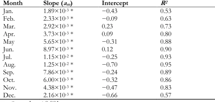
Table 2. Monthly results of linear regression between the biases and elevations of GPS stations.

Month Slope (am) Intercept R2

Jan. 1.89×10-3 _{* −0.43 0.53}

Feb. 2.33×10-3 _{* −0.09 0.63}

Mar. 2.92×10-3 _{* 0.23 0.73}

Apr. 3.73×10-3 _{* 0.09 0.80}

May 5.65×10-3 _{* −0.31 0.88}

Jun. 8.97×10-3 _{* 0.12 0.90}

Jul. 1.15×10-2 _{* −0.25 0.93}

Aug. 1.25×10-2 _{* −0.70 0.95}

Sep. 7.86×10-3 _{* −0.24 0.89}

Oct. 6.00×10-3 _{* −0.32 0.86}

Nov. 4.38×10-3 _{* −0.47 0.83}

Dec. 2.16×10-3 _{* −0.66 0.57}

*: p-value < 0.001.

4.2. Validation of Elevation-Corrected PW

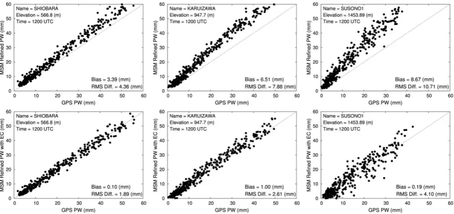
According to the procedure explained in Section 3.2, MSM-refined PW in 2014 was estimated at 3-h intervals and then corrected for elevation using Eq. (14). The elevation-corrected MSM-refined PW values were compared with the GPS PW at each GPS station. Figures 5 and 6 show the scatter plots between MSM-refined PW with/without elevation correction and GPS PW at the validation sites at 0000 and 1200 UTC in 2014, respectively. These figures show that the MSM-refined PW at each validation site agreed well with the GPS PW after elevation correction.

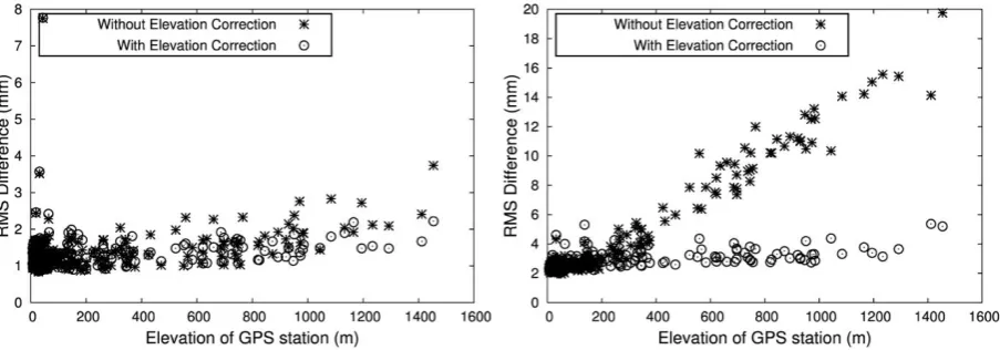
Figure 7 shows the scatter plots between the monthly RMS difference of PW at each GPS station and the elevation of each GPS station. The left and right panels in Fig. 7 show the relationships between RMS difference and elevation at the GPS stations in January and August of 2014, respectively. The RMS difference at each GPS station showed no dependence on elevation; thus, we can conclude that elevation correction removed the elevation dependence of bias and RMS difference at almost all the GPS stations. However, the RMS difference increased after elevation correction at some GPS stations located in the lower-elevation region. As shown in Fig. 4, the bias at lower-elevation (less than approximately 200 m) GPS stations did not fit well to the regression line. Overcorrection may have occurred at these GPS stations.

We also calculated the daily biases and RMS differences between MSM-refined PW and GPS PW at all GPS stations. Figure 8 shows the annual variation in daily bias and daily RMS difference in 2014. The blue line in Fig. 8 represents the annual variation in daily bias and RMS difference between elevation-corrected MSM-refined PW and GPS PW, and the red line represents the annual variation in daily bias and RMS difference without elevation correction. Without elevation correction, the RMS difference exceeded 4.0 mm on almost every day from June to September. This RMS difference was reduced to within 4.0 mm throughout the year by elevation correction.

MSM-refined PW decreased in the higher-elevation region, and high-resolution distribution of atmospheric water vapor content could be estimated especially in that region.

Fig. 5. Scatter plots between MSM-refined PW with (lower row) and without (upper row) elevation correction and GPS PW at validation sites at 0000 UTC in 2014.

Fig. 7. Relationship between RMS difference of PW and elevation of GPS stations in January (left) and August (right) of 2014.

Fig. 8. Variations in daily bias (left) and daily RMS difference of PW (right) in 2014.

5.

Conclusion

In this study, we estimated the PW distribution at high spatial resolution using NWP and DEM data from the Kanto region of Japan. The PW distribution at 90-m resolution was estimated by integrating the specific humidity between the layers bounded by each pressure level of MSM GPV data while accounting for the difference in surface elevation within pixels of MSM GPV data using 90-m-resolution ASTER GDEM data. The PW distribution was then corrected for elevation using the monthly slopes of linear regression lines between the biases and elevations of GPS stations. Elevation correction was necessary because the large elevation differences between MSM topography and GPS stations resulted in large biases between MSM-refined PW and GPS-derived PW. The results indicate that the proposed method can be used to estimate the PW distribution at a resolution of 90 m with an RMS difference of less than approximately 4.0 mm throughout the year. The method can provide high-resolution information on atmospheric water vapor content and its variation at 3-h intervals. This information is expected to be useful in climate research and for the atmospheric correction of remote sensing data, which can improve the accuracy of remote sensing measurements. Elevation correction resulted in the overestimation of PW at some lower-elevation GPS stations, which was attributed to overcorrection. Future work will identify the elevations at which elevation correction should be applied. In addition, the proposed method requires the monthly estimation of PW to obtain the monthly slope for elevation correction. Thus, this method cannot estimate PW in near-real time after obtaining MSM GPV data. Future work will also examine whether the slope values given in Table 2 vary by year. If the slope values vary little from year to year, they can be used in elevation correction to estimate the 90-m-resolution PW distribution in near-real time after obtaining MSM GPV data.

Acknowledgments

This study was supported by JSPS KAKENHI Grant Number 16K14298 and 17K01822.

References

[1] K. P. Czajkowski, S. N. Goward, D. Shirey, and A. Walz, “Thermal remote sensing of near-surface water vapor,” Remote Sens. Environ., vol. 79, no. 2-3, pp. 253-265, Feb. 2002.

[2] A. Dai, “Recent climatology, variability, and trends in global surface humidity,” J. Climate, vol. 19, no. 15, pp. 3589-3606, Apr. 2006.

[3] Y. Kinoshita, M. Furuya, T. Hobiger, and R. Ichikawa, “Are numerical weather model outputs helpful to reduce tropospheric delay signals in InSAR data?,” J. Geodes., vol. 87, no. 3, pp. 267-277, Mar. 2013. [4] J. Foster, B. Brooks, T. Cherubini, C. Shacat, S. Businger, and C. L. Werner, “Mitigating atmospheric

noise for InSAR using a high resolution weather model,” Geophys. Res. Lett., vol. 33, no. 16, Aug. 2006. [5] D. Cimini, N. Pierdicca, E. Pichelli, R. Ferretti, V. Mattioli, S. Bonafoni, M. Montopoli, and D.

Perissin, “On the accuracy of integrataed water vapor observation and the potential for mitigating electromagnetic path delay error in InSAR,” Atmos. Meas. Tech., vol. 5, no. 5, p. 1015, May 2012. [6] F. Onn, and H. A. Zebker, “Correction for interferometric synthetic aperture radar atmospheric phase

artifacts using time series of zenith wet delay observations from a GPS network,” J. Geophys. Res., vol. 111, no. B9, Sep. 2006.

[7] V. Cuomo, V. Tramutoli, N. Pergola, C. Pietrapertosa, and F. Romano, “In place merging of satellite based atmospheric water vapour measurements,” Int. J. Remote Sens., vol. 18, no. 17, pp. 3649-3668, Sep. 2006.

[8] M. Bevis, S. Businger, T. A. Herring, C. Rocken, R. A. Anthes, and R. H. Ware, “GPS meteorology: Remote sensing of atmospheric water vapor using global positioning system,” J. Geophys. Res., vol. 97, no. D14, pp. 15787-15801, Oct. 1992.

[9] T. Nilsson and G. Elgered, “Long-term trends in the atmospheric water vapor content estimated from ground-based GPS data,” J. Geophys. Res., vol. 113, no. D19, Oct. 2008.

[11] D. Perissin, E. Pichelli, R. Ferretti, F. Rocca, and N. Pierdicca, “Mitigtion of atmospheric water-vapor effects on spaceborne interferometric SAR imaging through the MM5 numerical model,” PIERS

ONLINE., vol. 6, no. 3, pp. 262-266, 2010.

[12] K. P. Czajkowski, S. N. Goward, S. J. Stadler, and A. Walz, “Thermal Remote Sensing of Near Surface Environmental Variables: Application Over the Oklahoma Mesonet,” The Prof. Geographer, vol. 52, no 2, pp. 345-357, May 2000.

[13] Z. Li, J. P. Muller, P. Cross, and E. J. Fielding, “Interferometric synthetic aperture radar (InSAR) atmospheric correction: GPS, Moderate Resolution Imaging Spectroradiometer (MODIS), and InSAR integration,” J. Geophys. Res., vol. 110, no. B3, Mar. 2005.

[14] R. Haas, J. G. Elgered, L. Gradinarsky, and J. Johansson, “Assessing long term trends in the atmospheric water vapor content by combining data from VLBI, GPS, radiosondes and microwave radiometry,” in Proceedings of the 16th _{Working Meeting on European VLBI for Geodesy and Astronomy, 2003,}

pp. 279-288.

[15] Research Institute for Sustainable Humanosphere, Kyoto University. (2017). Data form Japan

Meteorological Agency [Online]. Available: http://database.rish.kyoto-u.ac.jp/arch/jmadata/ [Accessed:

27 April 2017]

[16] Jet Propulsion laboratory, NASA. (2017). ASTER Global Digital Elevation Map Announcement [Online]. Available: https://asterweb.jpl.nasa.gov/gdem.asp [Accessed: 1 May 2017]

[17] University of Wyoming. (2017) Atmospheric Soundings - Wyoming Weather Web [Online]. Available: http://weather.uwyo.edu/upperair/sounding.html [Accessed: 27 April 2017]

[18] J. D. Means, “GPS precipitable water as diagnostic of the North American monsoon in California and Nevada,” J. Climate, vol. 26, no. 4, pp. 1432-1444, Feb. 2013.

[19] S. Vey, R. Dietrich, A. Rülke, and M. Fritsche, “Validation of precipitable water vapor within the NCEP/DOE reanalysis using global GPS observation from one decade,” J. Climate, vol. 23, no. 7, pp. 1675-1695, Apr. 2010.

[20] M. Shangguan, S. Heise, M. Bender, G. Dick, M. Ramatschi, and J. Wickert, “Validation of GPS atmospheric water vapor with WVR data in satellite tracking mode,” Ann. Geophys., vol. 33, no. 1, pp. 55-61, Jan. 2015.

[21] O. Bock, C. Keil, E. Richard, C. Flamant, and M. N. Bouin, “Validation of precipitable water from ECMWF model analyses with GPS and radiosonde data during the MAP SOP,” Q. J. R. Meteorol. Soc., vol. 131, no. 612, pp. 3013-3036, Oct. 2005.

[22] O. A. Alduchov and R. E. Eskridge, “Improved Magnus form approximation of saturation vapor pressure,” J. Appl. Meteorol., vol. 35, no. 4, pp. 601-609, Apr. 1996.

[23] T. Sakai, K. Koremura, and K. Niimi, “Height measurement error of barometric altimeter and its correction,” ENRI Papers, no. 114, pp. 1-13, Mar. 2005.

[24] S. Jan, D. Gebre-Egziabher, and T. Walter, “Improving GPS-based landing system performance using an empirical barometric altimeter confidence bound,” IEEE. Trans. Aerosp. Electron. Syst.., vol. 44, no. 1, pp. 127-146, Jan. 2008.

[25] R. J. Ross and W. P. Elliott, “Tropospheric water vapor climatology and trends over North America: 1973-93,” J. Climate, vol. 9, no. 12, pp. 3561-3574, Dec. 1996.

[26] J. Shuanggen, Z. Li, and J. Cho, “Integrated water vapor field and multiscale variations over China from GPS measurements,” J. Appl. Meteor. Clim., vol. 47, no. 11, pp. 3008-3015, Nov. 2008.

[27] H. Wang, M. Wei, G. Li, S. Zhou, and Q. Zeng, “Analysis of precipitable water vapor from GPS measurements in Chengdu region: Distribution and evolution characteristics in autumn,” Adv. Space