Rochester Institute of Technology
RIT Scholar Works
Theses Thesis/Dissertation Collections
8-15-2014
Unbalanced Workload Allocation in Large
Assembly Lines.
Christian E. Lopez
Follow this and additional works at:http://scholarworks.rit.edu/theses
This Thesis is brought to you for free and open access by the Thesis/Dissertation Collections at RIT Scholar Works. It has been accepted for inclusion
in Theses by an authorized administrator of RIT Scholar Works. For more information, please [email protected].
Recommended Citation
R.I.T.
Unbalanced Workload Allocation in Large
Assembly Lines.
by
Christian E. Lopez B.
A Thesis Submitted in Partial Fulfillment of the
Requirements for the Degree of Master of Science in Industrial
Engineering.
Department of Industrial and Systems Engineering
Kate Gleason College of Engineering
Rochester Institute of Technology
Rochester, NY
Department of Industrial and Systems Engineering
Kate Gleason College of Engineering
Rochester Institute of Technology
Rochester, NY
CETIFICATE OF APPROVAL
M.S. Degree Thesis
The M.S. Degree Thesis of Christian E. Lopez B.
has been examined and approved by the thesis
committee as satisfactory for the thesis
requirements for the Master of Science degree
Approved by:
Brian Thorn, Ph.D.
Scott Grasman, Ph.D.
Acknowledgements
I would like to extend my appreciation to the many people who helped to bring this research
project to completion. I would never have been able to finish my thesis without the guidance of
my advisors, help from friends, and support from the professor sand staffs of the Industrial
Systems Engineering department of RIT, especially Professor John Kaemmerlen and Marilyn
Houck.
First, I would like to thank Dr. Andres Carrano for providing me the opportunity of taking part in
the Master of Science program. I am so thankful for his help and valuable guidance. I would also
like to thank Dr. Brian Thorn and Dr. Scott Gasman for guiding my research for the past several
ii
Abstract
In modern production systems that perform under high cost environments, even small
improvements in line efficiency represents large savings over the lifetime of an assembly line. In
the beginning of modern production systems, it was thought that a ‘perfectly balanced’ line was
the most efficient way to design the line. However in practice, the ideal perfectly balancedline
seldom occurs, because some degree of imbalance is inevitable.
Recent studies have found that unbalanced lines with a bowl shape workload configuration can
yield performance in throughput as good as, or even better than those of a perfectly balanced
line. This thesis studied the “bowl phenomenon” in large unpaced assembly lines under
stochastic processing times. The control variables analyzed in this study were line length, buffer
capacity, task time variability, and percentage of imbalance. A full factorial experiment was
designed in order to characterize the main and interaction effects, and computational simulation
was used to replicate the behavior of the unbalanced assembly lines. The results of the
experiment suggest that unbalancing a large assembly line in a bowl shape workload
configuration could provide statistical significant improvements in throughput. Moreover, the
results also suggest that the Work in Process (WIP) and the Cycle Time (CT) increase linearly as
the Throughput (TR) of the line increases. Even though, the rate at which the TR increases is
greater than the rate at which the WIP and CT increases, line designers and production managers
need to make an important managerial decision on how much they are willing to increase the
WIP and CT of their lines in order to improve the throughput when implementing a bowl shape
workload configuration. Furthermore, the results suggested that as the buffer capacity and the
iii
increases the benefits the bowl phenomenon and the percentage of imbalance of the “best bowl
configuration” increases.
In this research, the relationship between the production rate of large assembly lines with a bowl
shape workload configuration and its line length, buffer capacity, task time variability, and
percentage of imbalance has been studied for the first time. The results would provide valuable
iv
Contents
List of Figures ... v
List of Tables ... vi
1. Introduction ... 1
2. Background ... 3
2.1. Simple Assembly Line Balancing Problem ... 3
2.2. Generalized Assembly Line Balancing Problem ... 5
2.3. Definitions ... 7
3. Literature Review ... 11
3.1. Assembly Line Balancing ... 11
3.2. Unbalanced Assembly Lines ... 15
3.3. The Bowl Phenomenon ... 17
3.4. Literature Gap ... 27
3.5 Research Questions ... 28
4. Proposed Methodology ... 30
4.1. Control and Response Variable ... 31
4.2. Line Design for Bowl Configurations ... 31
4.3. Line Design for Multiple Bowl Configurations ... 33
4.4. Preliminary Simulation Model ... 34
4.4.2. Simulation Run Parameters... 35
4.4.3. Model Validation ... 40
4.5. Data Analysis ... 48
5. Results and Discussion ... 50
5.1. One Bowl configuration ... 50
5.2. Multiple Bowl configuration ... 70
6. Summary and Conclusions ... 78
6.1. Summary ... 78
6.2. Conclusions ... 79
6.3 Future work ... 82
v
List of Figures
Figure 1.Precedence Graph ... 4
Figure 2.Workload distribution. ... 8
Figure 3. Example of traditional assembly line with buffer spaces. ... 8
Figure 4. Example one of Percentage of Imbalance ... 9
Figure 5. Example two of Percentage of Imbalance ... 10
Figure 6. Mechanics of the Flow Index ... 15
Figure 7. Two-level bowl configuration ... 19
Figure 8. Multi-level bowl configuration ... 19
Figure 9. Percentage decrease in mean output interval (Pike & Martin 1994) ... 23
Figure 10. Preliminary Simulation Model (3 workstation line) ... 35
Figure 11. Autocorrelation Function for WIP ... 37
Figure 12. Half width of the 99% CI under different number of simulation replications ... 39
Figure 13: Normal task time distribution, CV= 0.25 and B= 0... 41
Figure 14: Normal task time distribution, CV= 0.25 and B= 1... 41
Figure 15: Normal task time distribution, CV= 0.25 and B= 2... 42
Figure 16: Normal task time distribution, CV= 0.25 and B= 3... 42
Figure 17. Scenarios with Exponential task time distribution, CV=1, N=7-9 and B=0 ... 43
Figure 18. Scenarios with Exponential task time distribution, CV=1, N=3, and B=5, 10 and 15 ... 44
Figure 19. Scenarios withExponential task time distribution, CV=1, N=4-7, and B=0-5 ... 45
Figure 20. Scenarios with Erlang task time distribution, k=2-16, N=3, and B=0-5 ... 46
Figure 21. Scenarios with Erlang task time distribution, k=2-4, N=4-6, and B=0-4 ... 47
Figure 22. Minitab Summary of Error ... 48
Figure 23.Scatter plot Diagram %TR vs, % CT, and 5 WIP (B=0) ... 54
Figure 24.Scatter plot Diagram %TR vs, % CT, and 5 WIP (B=1) ... 54
Figure 25.Scatter plot Diagram %TR vs, % CT, and 5 WIP (B=2) ... 54
Figure 26.Main Effects Plot for throughput (One bowl configuration) ... 64
Figure 27. Interaction Plots for throughput (One bowl configuration) ... 64
Figure 28. Interaction Plots for throughput, CV vs. x. (One bowl configuration) ... 64
Figure 29.Interaction Plots for throughput, B vs. x. (One bowl configuration) ... 64
Figure 30.Interaction Plots for throughput, N vs. x. (One bowl configuration) ... 64
Figure 31. Residual Plots of the ANOVA for throughput (One bowl configuration) ... 65
Figure 32. Residual Plots of regression analysis. ... 69
Figure 33. Main Effects Plot for throughput (Two bowl configuration) ... 76
Figure 34. Interaction Plots for throughput (Two bowl configuration) ... 76
Figure 35. Interaction Plots for throughput, CV vs. x. (Two bowl configuration) ... 76
Figure 36. Interaction Plots for throughput, B vs. x. (Two bowl configuration) ... 76
Figure 37. Interaction Plots for throughput, N vs. x. (Two bowl configuration ... 76
vi
List of Tables
Table 1: Task Information ... 4
Table 2: Versions of SALBP ... 5
Table 3: Nomenclatures ... 7
Table 4: Percentage decrease in mean output interval (Pike & Martin 1994) ... 23
Table 5: Example of a 0 bowl configurations for assembly lines with N=10 ... 33
Table 6: Independent variable values for multi bowl configurations test ... 34
Table 7: 10 simulation replications data ... 38
Table 8: 30 simulation replications data ... 38
Table 9: 20 simulation replications data ... 38
Table 10: 40 simulation replications data ... 38
Table 11: Scenarios with Exponential task time distribution, CV=1, N=7-9 and B=0 ... 43
Table 12: Scenarios with Exponential task time distribution, CV=1, N=3, and B=5, 10,15 ... 44
Table 13: Scenarios withExponential task time distribution, CV=1, N=4-7, and B=0-5 ... 44
Table 14: Scenarios with Erlang task time distribution, k=2-16, N=3, and B=0-5 ... 45
Table 15: Scenarios with Erlang task time distribution, k=2-4, N=4-6, and B=0-4 ... 46
Table 16.Minitab One-Sample T-test... 48
Table 17. Assembly lines simulated with one bowl configuration ... 52
Table 18.Correlation Analysis TR vs WIP ... 53
Table 19. 95% CI of the throughput for the lines with one bowl shape and CV of 0.2 ... 55
Table 20. 95% CI of the throughput for the lines with one bowl shape and CV of 0.8 ... 56
Table 21. 95% CI of the throughput for the lines with one bowl shape and CV of 1.4 ... 57
Table 22. 95% CI of the WIP for the lines with one bowl shape and CV of 0.2 ... 58
Table 23. 95% CI of WIP for the lines with one bowl shape and CV of 0.8 ... 59
Table 24. 95% CI of the WIP for the lines with one bowl shape and CV of 1.4 ... 60
Table 25. Percentage of Potential Improvement (Robustness) ... 61
Table 26. Analysis of Variance for throughput (One bowl configuration) ... 62
Table 27. Stepwise Regression ... 66
Table 28. Regression analysis for percentage of improvement in throughput . ... 68
Table 29. Assembly lines simulated with two bowl configuration ... 70
Table 30. 95% CI of the throughput for the lines with two bowl shape configuration ... 72
Table 31. 95% CI of the WIP for the lines with two bowl shape configuration ... 73
Table 32. Paired T-test for the “best two bowl configuration” (CV=14, B=2, and N=70) ... 74
1
1.
Introduction
Assembly lines are key components of modern production systems. The first real example of an
assembly line is attributed to Henry Ford, with the assembly line of the Ford Model T in 1913. In
the beginning of modern production systems, it was thought that a ‘perfectly balanced’ line
(equal workload along all workstations) was the most efficient way to design the line. This
stimulated a great amount of research in heuristic and near optimal algorithms for the Assembly
Line Balancing Problem (ALBP) that aimed for the perfectly balanced workload allocation.
The design and planning of production systems is a vital task for line designers and production
managers. In modern production systems that perform under high cost environments, even small
improvements in line efficiency represents large savings over the lifetime of an assembly line. In
practice, the ideal perfectly balancedline seldom occurs, because some degree of imbalance is
inevitable. A perfectly balanced line might not be possible due to some technological and/or
organizational constraints, task variability or due to the performance rate of workers.
Recent studies have found that unbalanced lines, in which workstations have different
workloads, can yield performance as good as, or even better than those of a perfectly balanced
line. The “bowl configuration” of workload, in which greater workload is allocated towards the
ends of the lines and decreasingly less in a symmetric pattern toward the center, have been
shown to improve the production rate of assembly lines. Since the discovery of the “bowl
phenomenon” numerous studies have been done to understand its benefits. Even though
assembly lines consist of hundreds or even of thousands of tasks, and a large number of
workstations, many research efforts done on the bowl phenomenon have not experimented with
2
This thesis aims to study the “bowl phenomenon” in large unpaced assembly lines under
stochastic processing times. This will improve the understanding of the relationship between the
production rate of assembly lines with a bowl shape workload configuration and its line length,
buffer capacity, and task time variability. Furthermore, it will provide valuable guidelines for
line designers and managers to improve their production systems. Section 2 provides a
background; section 3 is a detailed review of existing literature of balanced and unbalanced
assembly lines, and outlines the research questions. In section 4 the methodology used in this
study is presented. Furthermore, in section 5 the results of the experiments are provided, and in
3
2.
Background
2.1. Simple Assembly Line Balancing Problem
The problem of planning for the allocation of work elements into assembly lines has been the
subject of interest for a long time. According to Baybars (1986) the first analytical statement of
the Assembly Line Balancing Problem (ALBP) in a mathematical form was published by
Salveson (1955).
Assembly lines can be defined as a finite set of workstations arranged along material handling
equipment. Workpieces are successively passed down the assembly line and moved from one
workstation to the next. To produce any product on an assembly line it is required to divide the
total amount of work into a finite set of elementary tasks. Performing a particular operation
requires a task time, and certain equipment and/or skilled workers. The total workload necessary
to assemble a workpiece is calculated by the sum of all the task times Due to some technological
and/or organizational conditions, the precedence constraints between tasks need to be taken into
consideration at the moment of assigning the elementary tasks to the workstations on the line.
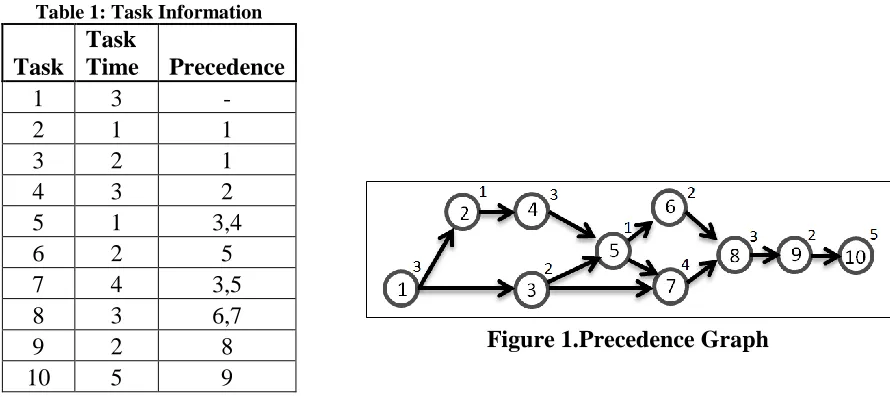
These constraints can be visualized in a precedence graph. A precedence graph contains a node
for each task, a node weights for the task times, an arcs for the direct precedence constraints (see
Table 1), and a paths for the indirect precedence constraints. For example, in Figure 1 task# 6
and #7 needs to be completed after starting task #8. This precedence graph contains a set of 10
4
Table 1: Task Information
Task
Task
Time Precedence
1 3 -
2 1 1
3 2 1
4 3 2
5 1 3,4
6 2 5
7 4 3,5
8 3 6,7
9 2 8
10 5 9
Figure 1.Precedence Graph
The fundamental objective of ALBP is the assignment of tasks to an ordered sequence of
workstations, such that the precedence relations and other constraints are not violated and some
measure of effectiveness is optimized. Most of the research done in assembly lines has focused
on solving the Simple Assembly Line Balancing Problem (SALBP) (Scholl and Becker, 2006).
This type of the ALBP is based on the following assumption (Baybars, 1986):
The line is designed for a unique model of a single product
Deterministic task times
A task cannot be split among two or
more stations
There are no assignments restrictions beside the precedence constraints.
All tasks must be processed
All workstations are equally equipped
The line has a serial layout with N one-sided workstations.
All these assumptions reduce the complexity of the problem. However, the balancing of real
assembly lines requires the consideration of additional technical and/or organizational
constraints, which increases the complexity of the problem. There exist four different versions of
5
Table 2: Versions of SALBP
(Scholl and Becker, 2006)
Cycle Time
Given Minimize
Number of workstations
Given SALBP-F SALBP-2
Minimize SALBP-1 SALBP-E
SALBP-F is a feasibility problem that is objective is to establish whether or not a feasible line
balance exists for a given combination of workstations and cycle time. SALBP-1 aims to
minimize the number of workstations given a fixed cycle time. SALBP-2 aims to minimize the
cycle time given a set of workstations. SALBP-E is the most general version of the problem; it
aims to maximize the line efficiency by simultaneously minimizing cycle time and the number of
workstations.
2.2. Generalized Assembly Line Balancing Problem
Balancing of real assembly lines requires considering additional technical and/or organizational
constraints, in contrast with the SALBP. Any ALBP that does not follow all the assumption of
the SALBP are considered Generalized Assembly Line Balancing Problems (GALBP) (Baybars,
1986). One of the main assumptions of the SALBP is that all processing times are known with
certainty (deterministic task times). In assembly lines with highly automated workstations,
where tasks time variance is sufficiently small, the tasks time might be considered to be
deterministic. However, when human operations are involved, the variance of the processing
times increases. This is generally attributed to the variability of humans with respect to work
rates, skill, and motivation levels (Becker and Scholl, 2006).
The stochastic version of the GALBP introduces the concept of task time variability. When
6
SALBP. Under stochastic processing times, workstations could finish their work in different
periods. To accommodate for this variability buffer spaces can be allocated between
workstations. Furthermore, the launch rate of the workstations could be controlled to either be
paced or unpaced.
In paced assembly lines systems a common cycle time limits the processing times of all the
workstations. This is achieved either by continuous or intermittent conveyor belts, which force
the operators to finish the tasks before the workpiece reaches the end of the workstation. If
continuous material handling equipment is used to pace the line, the workstations length needs to
be defined taking in consideration the workload configuration of the line.
In contrast, unpaced lines are not limited to a given time span to transfer the workpieces.
Therefore, production rates are no longer given by a fixed cycle time. Some authors classify
unpaced lines in asynchronous and synchronous unpaced lines. In asynchronous unpaced lines
the workpieces are always moved whenever the required operations are completed, and if the
following workstation is not blocked by another workpiece. After transferring the workpiece the
workstation continues to work, unless the preceding workstation is unable to deliver a new
workpiece. When this happens the workstation waiting for the new workpiece is considered to be
starved. In order to minimize the “blocking” and “starving” of workstations buffers capacity can
be implemented. In synchronous unpaced lines all workstations wait until the slowest one
finishes its work before the workpieces are transferred. In contrast to the asynchronous unpaced
lines, buffers between workstations are not required. Under deterministic processing time a
synchronous unpaced line works as an intermittent paced line, with the cycle time determined by
the slowest workstations. However, synchronous unpaced lines can transfer the workpieces if
7
2.3. Definitions
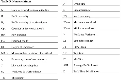
[image:16.612.67.558.155.482.2]In this section the general concepts used in this study are defined using the nomenclatures of Table 3.
Table 3: Nomenclatures
N Number of workstations in the line
B Buffer capacity
Bn Buffer capacity of workstation n
Opn Operator in the workstation n
RM Raw material
FG Finished goods
DI Degree of imbalance
MAD Mean absolute deviation of workload
tn Processing time of workstation n
T Line total operating time
wn Workload of workstation n
TR Throughput
c Cycle time
E Line efficiency
WR Workload range
Wmax Maximum workload
Wmin Minimum workload
V Workload Variance
SI Smoothness index
FI Flow index
TT Takt time
IT Idle Time
ABL Average Buffer Levels
D Task Time Distribution
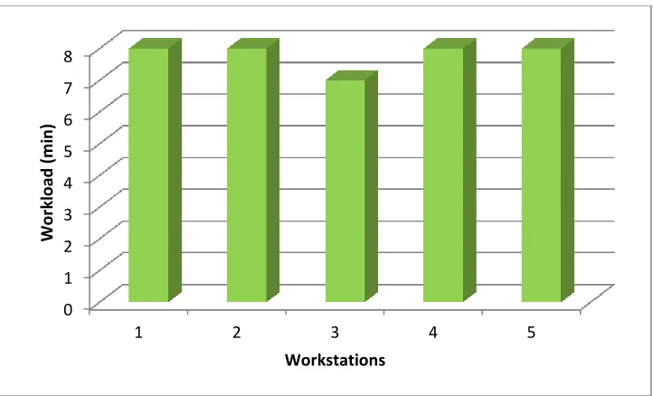
Workstation and Workload:
Assembly lines can be defined as a finite set of workstations arranged along a material handling
equipment. The workstation workload is the sum of all the tasks times allocated to that
8
Figure 2.Workload distribution
Buffers:
Buffers are physical locations used to temporarily store work in process (WIP) in the assembly
line. For an assembly line with a set of N workstations, there will be a total of N - 1 buffers,
represented as: B1, B2, B3,…,Bn-1. The buffer after workstation 1 is referred to as B1, the buffer
after the 2nd workstation as B2, and so on until the last buffer. The last buffer is referred to as
Bn-1. For example, Figure 3 shows a line with 3 workstations, 3 operators, and two buffer spaces
(B1 and B2).
WS1 WS2 WS3
RM B1 B2 FG
[image:17.612.126.487.69.288.2]Op1 Op2 Op3
Figure 3. Example of traditional assembly line with buffer spaces.
0
1 2 3 4 5 6 7 8
1 2 3 4 5
Wor
kl
o
ad
(
m
in
)
9
Degree of Imbalance:
The degree of imbalance (DI) of a line configuration is the percentage of workload imbalance. It
is measured by the mean absolute deviation of workload (MAD). (N is number of workstations in
the line, T is the line total operation time, and wn is the workload of workstation n).
∑ | ⁄ |
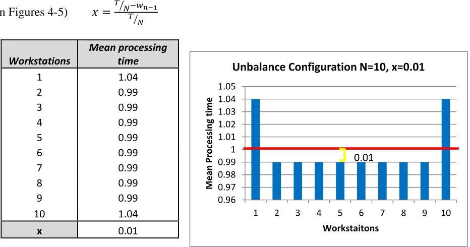
Percentage of Imbalance (x)
The Percentage of Imbalance is the percentage difference in mean processing time between the
inner workstations of a two level bowl configuration and its balanced counterparts. (See example
in Figures 4-5) ⁄ ⁄
Workstations
Mean processing time
1 1.04
2 0.99
3 0.99
4 0.99
5 0.99
6 0.99
7 0.99
8 0.99
9 0.99
10 1.04
[image:18.612.76.542.365.610.2]x 0.01
Figure 4. Example one of Percentage of Imbalance
0.96 0.97 0.98 0.99 1 1.01 1.02 1.03 1.04 1.05
1 2 3 4 5 6 7 8 9 10
M
e
an
Pr
o
ce
ssi
n
g
tim
e
Workstaitons
Unbalance Configuration N=10, x=0.01
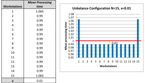
10 Workstations
Mean Processing time
1 1.065
2 0.99
3 0.99
4 0.99
5 0.99
6 0.99
7 0.99
8 0.99
9 0.99
10 0.99
11 0.99
12 0.99
13 0.99
14 0.99
15 1.065
[image:19.612.72.544.72.344.2]x 0.01
Figure 5. Example two of Percentage of Imbalance
Throughput:
Throughput (TR) is defined as the average output of a production process (machine, workstation,
line, plant) per unit time. Therefore, in an assembly line throughput is the average quantity of
nondefective parts produced in the line per unit time. The importance of using throughput as a
measurement of a production system is that it is the most frequently used measure by engineers
and managers when designing and operating a line. 0.95 0.96 0.97 0.98 0.99 1 1.01 1.02 1.03 1.04 1.05 1.06 1.07 1.08
1 2 3 4 5 6 7 8 9 10 11 12 13 14 15
M
e
an
p
ro
ce
ssi
n
g t
im
e
Workstations
Unbalance Configuration N=15, x=0.01
11
3.
Literature Review
3.1. Assembly Line Balancing
The fundamental ALBP seeks to assign tasks to an ordered sequence of workstations, such that
the precedence relations are not violated and some measure of effectiveness is optimized. The
measures of effectiveness used in ALBP can be divided into two categories: economic and
technical measures (Ghosh & Gagnon, 1989).
The use of economic measures could be encouraged by the impact in the profitability and
operational cost that the design and planning of assembly lines might have on an organization.
Many authors have implemented cost-oriented models to solve ALBP. Chakravarty (1985) and
Silverman (1986) implemented heuristics that focused on minimizing the total cost of the line,
while Askin (1997) implemented a heuristic that focused on minimizing the operational and
equipment cost of the line. Rosenberg (1992) made the assumption that the operation of a
workstation causes a wage rate that was directly related to the maximum wage rate of all tasks
that are assigned to that workstation. The objective was to minimize the aggregate wage rate over
all workstations, which was equivalent to minimizing the number of workstations in the case that
all tasks have the same wage rates. Amen (2000) extends Rosenberg’s heuristic by adding a cost
of capital, which could be explained as the initial investment cost for the workstations.
Since ALBPs have a long to mid-term planning horizon, the criteria used to measure the
effectiveness of the lines need to be carefully selected considering the strategic goals of the
organization. From an economic point of view profitability and cost measures are preferable.
12
profits achieved by selling the products assembled is moderately complicated and error prone.
These might be the reasons why technological measures are more popular in the ALBP (Becker
& Scholl, 2006)
The technological measures commonly used are related to the throughput and/or operational
efficiency of the assembly lines. Many authors have used the line efficiency as an indicator for
operational efficiency (Scholl et al., 2006). McMullen (1997), Macaskill, (1972) and Gokcen et
al. ( 1999) used line efficiency in their heuristic for solving the mixed-model assembly line
balancing problem. Line efficiency (E), consists in maximizing the line utilization which is
measured as the productive fraction of the line total operating time (T) over the cycle time (c)
and the number of workstations (N). The maximization of the line efficiency is a measure that
directly addresses the minimization of workstations and the idle time of the line.
⁄
The primary objective of the line designer should be to minimize the number of workstations,
and as a secondary objective to distribute the amount of workload as evenly as possible among
the workstations (Talbot, 1991). Although, Sparling (1998), Miltenburg (1998), Sabuncuoglu
(2000), and Kara (2007) had the minimization of workstation as the primary objective, the
minimization of workload differences among the workstations was a secondary objective.
There are many criteria which can be used to optimize the distribution of workload among the
workstations on a line. The workload range (WR) measures the extreme values of the workloads
13
difference between the maximum (Wmax) and the minimum workload (Wmin) of the
workstations on an assembly line.
WR= Wmax - Wmin
The workload variance (V) penalizes deviations from the mean workload quadratically (N is the
total number of workstations, T is the line total operating time, and wn is the workload of
workstation n).
∑ ⁄
Moreover, the mean absolute deviation of workload (MAD) penalizes deviations from the mean
workload linearly.
∑ | ⁄ |
As Talbot (1991) explained, workload variance and mean absolute deviation of workload are
very similar, and from a practical perspective there may be no reason to choose one criteria over
the other. However, an important consideration is to select a criterion that allows constructing
tractable linear measurements to compare different line balance designs. This linear tractable
property is the reason why Talbot (1991) used the MAD as the criterion to measure the workload
distribution in his assembly line balancing algorithm.
Baybars (1986) suggested that ALBP could be improved by adding a secondary objective which
consists of smoothing the overall workstations workloads. The smoothness index (abbreviated SI
14
smoothness index is the root square of all the square differences between the cycle time (c) and
the workstations workload ( .
√∑
The primary objective of the assembly line designers usually is the minimization of workstations
or the maximization of line efficiency, while workload balance is a secondary objective. The
main reason for this is that as the number of workstations in a line increases the overall cost also
increases. Moreover, to achieve the maximum potential of an assembly line its efficiency should
be 100%. However, in the case that 100% efficiency is not possible (due to some technological
and/or organizational constraints), it was thought that the flow of the line, the output rate, the
lead time, and work in progress (WIP) were optimized by reducing the workload differences
among workstations.
Kathiresan et al. (2012) presented a method that assigned work elements to workstations with a
criterion to meet takt time and achieved workload balance among workstations. They introduce a
new line efficiency criterion called flow index (FI), which penalizes deviation of workstation
workload ( from the takt time of the line (TT). By minimizing the flow index the workload
smoothness among workstations with respect to takt time is reduced. They defined the flow
index as the root mean square of deviation of workstations workload and takt time.
√
15
The value of the flow index varies from 0 to 1. A flow index of ‘zero’ indicates a perfectly
balanced line, and a value of ‘one’ indicates the greatest possible difference between
workstations workload and the takt time of the line (extreme condition) (Figure 6). Therefore,
smaller values of flow index results in smooth workload distribution among the workstations
with respect to takt time.
Figure 6. Mechanics of the Flow Index
(Kathiresan, Jayasudhan, Prasad, and Mohanram, 2012)
3.2. Unbalanced Assembly Lines
Boysen et al. (2008) showed that the ALBP has been an important field of research since its first
analytical statement was published in 1955. All this research has built a significant body of
literature, which covers a lot of different aspects of a production system. However, they were
able to recognized only 15 articles which explicitly deal with ALBP of real world. In contrast to
the 312 different research publications treated in the latest literatures review of ALBP analyzed
in this survey(Scholl & Becker, 2006; Becker & Scholl, 2006; Boysen, Fliedner, & Scholl, 2006
). Those 15 articles represent less than 5% of the body of literature studied, which as the authors
highlighted is an indication of the noteworthy gap that exist between the current status of
research and the requirements of real world problems. Templemeir (2003) indicated that
16
great number of ALBP algorithms, which made the assumption of equal processing time over all
the workstations, are not appropriate for real world systems.
In real assembly lines task variability is present due to human labor, production mix and/or
machines breakdowns. In these lines different issues arise that are not considered in many ALBP
algorithms that make the assumption of deterministic task times. As stated by Ghosh and
Gagnon( 1989) when task variability is present new problems arise, such as the workstations
time exceeding the cycle time, the production of unfinished parts, the pacing effects on worker’s
processing times, the size and location of inventory buffers, launch rates, and allocation of the
workload along the line. So, under stochastic environments the line designers need to answer
questions regarding what cycle time to choose, how much and where buffers inventory should be
allocated or if planned imbalance should be considered into the system.
Planned imbalance means that workload of all workstations of the assembly line are intentionally
designed to be unbalanced and not necessarily equal to each other. According to Carnall and
Wild (1976) in real production systems a perfectly balance line may be impossible because:
1 .In most cases equal allocation of workload to workstations may be prevented by precedence
and/or technological constraints
2. The variability of the processing times at individual workstations may differ as a result of
differences in the nature of the tasks.
3. Individual workers may have different mean work performance rates.
Previous studies in unbalanced lines have concluded that, under real conditions, perfectly
17
showed statistically significant improvement on throughput of nearly 3%, on idle time of 32%,
and on average buffer levels of 90% by deliberately unbalancing the workload, buffer capacity
and variability of the workstations in the line. In modern production systems, that perform under
high cost environments, these improvements still represent a large saving over the lifetime of an
assembly line (Das et al. 2010). Thus, as stated by Hillier and So (1996) line designers should
concentrate more efforts on unbalancing the line in an optimal or near optimal configuration,
given that perfectly balanced lines are difficult to achieve and are ‘riskier’ targets.
3.3. The Bowl Phenomenon
The experimental results of Hillier and Boling (1966) were the first to highlight the benefits of
unbalancing the mean processing time in a bowl shape configuration , thus discovering the
existence of the ‘bowl phenomenon’. In this work a queuing model for lines length of up to 4
workstations (N=4) with exponential task time distributions was implemented to study the ALBP
in unpaced asynchronous lines with variable processing times. It was shown that the output rate
can be improved, compare to a balanced line, by deliberately unbalancing the line by allocating
higher and equal workload to the first and last workstations and lower workload to the middle
workstations.
Subsequent research done by Rao (1976), Carnall and Wild (1976), and De la Wyche et al.
(1977) also demonstrated the benefits and existence of the bowl phenomenon. Rao (1976)
experimented with 3 workstation assembly lines with different combinations of task time
distributions (exponential, uniform and deterministic). It was shown that in a three station system
the improvements in the throughput can be as large as 6.79%.In this study, it was demonstrated
18
workstations to the exterior ones (first and last workstation); preferably when the coefficient of
variation (CV) of the workstations is less than 0.5. Alternately, when the coefficient of variation
(CV) of the workstations is greater than 0.5 (CV>0.5) allocating the workload of the more
variable workstations to the less variable ones would provide a better configuration.
Carnall and Wild (1976) experimented with 4 and 10 workstations assembly lines, buffer
capacity of 1, 2 and 3 units , under a positively skewed Weibull task time distribution and
Coefficient of Variation of 0.1,0.21 and 0.5. In this study, by implementing a bowl shape
configuration it was possible to produce improvements in throughput up to 4% over the balanced
lines. These results confirmed the existence of the ‘bowl phenomenon’ and extended it to the
case of changing workstations variance rather than workload. It was also discovered that
increasing buffer capacity or reducing the CV of the workstations reduces the improvement of
unbalancing the line in a bowl shape configuration.
Hillier and Boling (1979) established general guidelines for the bowl configurations. These
guidelines were:
-The optimal bowl allocation should be symmetric.
-The optimal bowl allocation should be relatively flat in the middle and very steep towards the
end of the line.
-The degree of imbalance should decrease with the inter station buffer storage capacity.
-The degree of imbalance should increase with the length of the line.
19
Based on these general guidelines the line design may consist of a two-level bowl or a
multi-level bowl configuration. A two-multi-level bowls configuration consists of equal workload at the first
and last workstation of the line, with equal but smaller workload at all workstation in between. A
multi-level bowl configuration typically consists of greater workload at the first and Nth
workstation (Level 1), equal but smaller workload for the 2nd and (N-1)th workstations (Level
2), and successively smaller paired workload at the remaining workstations (Level 3). For
example, Figure 7 shows a two-level bowl configuration, in which workstations 1 and 6 are the
Level 1, and the remaining workstations (2-5) are the Level 2. Figure 8 shows a multi-level bowl
configuration, in which workstations 1 and 6 are the Level 1, workstations 2 and 5 are Level 2,
and workstations 3 and 4 are Level 3.
Figure 7. Two-level bowl configuration Figure 8. Multi-level bowl configuration
Hillier and Boiling (1979) provided the first extrapolation model for near optimal bowl
configurations, and demonstrated that as the number of workstations in the line increase from 2
to 6, under 0 buffer capacity and CV of 1, the degree of imbalance in the optimal bowl
configuration tends to stay the same. Moreover, the improvements in output rate become greater
as the line length increases. Also, when task time distributions are highly variable (Erlang and
Exponential distribution with CV>1) the degree of imbalance in the optimal bowl configuration 0
2 4 6 8 10 12 14
1 2 3 4 5 6
W
o
rklo
ad
(
mi
n
)
Workstations
0 2 4 6 8 10 12 14
1 2 3 4 5 6
W
o
rklo
ad
(
mi
n
)
20
substantially decreases as the buffer capacity increases, supporting previous studies of Hatcher
(1969), Quarles (1967), Sheskin (1976), Smith and Brumbaugh (1977) and Carnall and Wild
(1976) about the effect of inventory buffers in assembly line output rate.
El-Rayah (1979) presented the first study to use simulation to confirm the existence of the bowl
phenomenon. In this study, different unbalance configurations were simulated in assembly lines
with up to 12 workstations under Normal, Lognormal and Exponential task time distributions
and CVs of 0.3 and 1. It was demonstrated that the bowl configuration was the only one to
consistently improve the output rate, compared to the balanced line and the other unbalanced
configurations tested (ascending, descending, and “low-high-low-high”). But, more important
these results demonstrated that unbalancing a line in the wrong configuration might produce
negative outcomes.
An interesting experiment that used simulation and analytical models to study the unbalanced
stochastic assembly lines was presented by Smunt and Perkins (1985). It suggested that balanced
lines are as good as or better than unbalanced lines, when processing times are modeled under
more realistic values of task time variance. In this study, assembly lines with 3 and 4
workstations under Normal task time distribution and CV of 0.2, 0.5 and 1 were simulated. It
was concluded that unbalancing the lines should only be considered when task time distribution
has great variance. Furthermore, that more extensive experiment research with various normal
task time distribution and different workstations lengths should be conducted.
The conclusions of Smunt and Perking (1985) regarding the bowl phenomenon motivated that
Karwan and Philipoom (1989) published an article that highlighted the flaws of the previous
21
the small sample size. It was also stated that Smunt and Perking (1985) didn’t use Hillier and
Boling (1979) optimal bowl configurations. Finally, that Dudley’s (1963) and Knott and Sury’s
(1987) research clearly indicated that the frequency distribution of task times for experienced
workers on unpaced lines is positively skewed. Dudley mentioned that times for trainees or when
various interventions are designed to pace workers a Normal distribution is perhaps appropriate.
Muth and Alkaff (1987) demonstrated a method that analyzed serial production lines and
computed the output rate of assembly lines with unbalanced workstations. In this work, the
authors highlighted that an important characteristic of the Hillier and Boling (1979) study was
the use of fixed CV. Therefore, in the Hiller and Boling (1979) study it was not possible to select
the variance independently of the mean processing times of the tasks. This raised the question of
what really caused the bowl phenomenon, the change in service time variance or the changes in
mean processing time of workstations. Using an innovative method based on random
distributions, Muth and Alkaff (1987) demonstrated that carefully selected bowl configurations
do indeed provide some improvements over the balanced lines, when the sum of the total mean
processing times and variance are conserved.
So (1989) simulated 3, 4 and 8 workstation assembly lines with buffer capacity of 1,3 and 5
under Exponential task time distribution with CV=1, and Normal task time distribution with
CV= 0.2, 0.46 and 0.62. Based on the general guidelines of Hillier and Boling (1979), 4 different
bowl configurations were simulated. It was concluded that very small improvements (0.3% in
average) in the efficiency of an assembly line with finite buffer could be achieved if the line is
unbalanced properly. Therefore, in contrast with Smunt and Perking (1989) results, the authors
concluded that improvements in line efficiency could be achieved even when task time
22
Hillier and So (1993) improved the extrapolation procedure of Hillier and Boling (1979) by
implementing a new related measure of imbalance. In this study, assembly lines with 3 up to 9
workstations, buffer capacity of 0 up to 5 under Exponential and Erlang task time distributions
with CV of 0.25 up to 0.707, were simulated. The authors stated that this study was limited to
experiments with small assembly lines (N<9) due to computational requirements. However, it
was indicated that many real assembly line systems have a larger number of workstations, hence
the importance of extrapolating the “optimal bowl configuration” for larger assembly lines. The
study confirmed that the percentage of improvement increases as the number of workstations in
the line increases. For example, an assembly line with zero buffer capacity, Exponential task
time distribution and 7 workstations shows an improvement of 1.48%, while a line under the
same conditions but with 9 workstations shows an improvement of 1.59%.
Pike and Martin (1994) provided an extensive simulation and are the only ones to have studied
the bowl phenomenon in assembly line with up to 30 workstations. In this study, assembly lines
with 3-12, 15, 20, 25 and 30 workstations, buffer capacity 0-4 units under Normal and positively
skewed task time distributions with CV of 0.2, 0.25 and 0.30 were simulated. Different bowl
configurations were systematically tested with 0.001increments in the mean processing time of
the workstations until it performed more efficiently than the balanced line, according to paired
t-test at a 99.95% confidence level. The configuration with the statistically smaller mean output
interval was selected as the “optimal bowl configuration”. In this study, it was also shown that
the maximum degree of imbalance that would still yield a mean output interval that perform
statistically no worse than the balanced line. The authors were able to demonstrate that the bowl
phenomenon also exists for large assembly lines, with small CV (CV=0.2) values, and relatively
23
In this study, the effect of the line length over the bowl phenomenon was demonstrated. The
percentage values of improvement in mean output interval resulting from the use of optimal bowl
configuration, in assembly lines with Normal task time distribution and CV= 0.25, are shown in
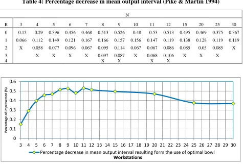
[image:32.612.70.545.187.510.2]Table 4 (N is the number of workstations in the line, B is the buffer capacity) and in Figure 9.
Table 4: Percentage decrease in mean output interval (Pike & Martin 1994)
N
B 3 4 5 6 7 8 9 10 11 12 15 20 25 30
0 0.15 0.29 0.396 0.456 0.468 0.513 0.526 0.48 0.53 0.513 0.495 0.469 0.375 0.367
1 0.066 0.112 0.149 0.121 0.167 0.166 0.157 0.156 0.147 0.119 0.138 0.128 0.119 0.119
2 X 0.058 0.077 0.096 0.067 0.095 0.114 0.067 0.067 0.086 0.085 0.05 0.085 X
3 X X X X 0.097 0.087 X 0.068 0.106 X X X
4 X X X X
Figure 9. Percentage decrease in mean output interval (0 buffer capacity, CV of 0.25 and normal task time distribution) (Pike & Martin 1994)
In Figure 9 it can be observed that the percentages of improvement of the bowl phenomenon
rapidly increases as the number of the workstations reaches to 12. This supports the conclusion
of Hillier and Boling (1979), that the improvement in production rate becomes greater as the line
length increases. However, for lines larger than 12 workstations it showed a tendency to reduce
the percentage of improvements. 0
0.1 0.2 0.3 0.4 0.5 0.6
3 4 5 6 7 8 9 10 11 12 13 14 15 16 17 18 19 20 21 22 23 24 25 26 27 28 29 30
Per
ce
nt
ag
e
o
f
imp
ro
ve
mn
t
(%
)
Workstations
24
Many studies have proven the existence and potential benefits of the bowl phenomenon.
However, the benefits that could be achieved by deliberately unbalancing a line with a bowl
configuration depend on correctly identifying the line parameters in order to estimate the best
bowl shape configuration. Regardless of the proven improvements that the bowl phenomenon
provides, perfectly balanced lines remain the norm of the industry (Hillier & So, 1996). A
frequently stated reason for this is the uncertainty about the robustness of the bowl phenomenon
(Smunt & Perkins, 1989). Hillier and So (1996) studied the robustness of the bowl phenomenon
by experimenting with the effects that a poor estimation in the amount of imbalance of the bowl
configurations would have over the throughput of the line. In this study, experimental results
demonstrated that the bowl phenomenon is relatively robust, because even larger error (50%) in
the degree of imbalance of the “optimal bowl configuration” would still provide most of the
potential improvement in output rate. Furthermore, the output rate still exceeds the one of a
balanced line in most cases even when the workload configuration deviates from the optimal
bowl by 10%. It was concluded that unbalanced lines provided a more robust target than the
perfectly balanced lines, which are ‘riskier’ targets.
Hillier et al. (2006) studied both workload and buffer bowl configurations. In this study a cost
oriented model, which takes into account the revenue per unit of output and the cost per unit of
buffer space, was implemented. Assembly lines with 4 and 5 workstations, under Exponential
and Erlang task time distributions with relatively large variance were simulated. The results
showed that both of the buffer and workload bowl configuration were very similar. It was
concluded that this same pattern would hold for larger lines. The improvement achieved by just
optimizing the workload allocation in a bowl configuration and balanced buffer allocation was
25
Shaaban and McNamara (2009) did an extensive simulation and statistical analysis to study
unbalanced workload allocation in non-automated production lines. In this study, assembly lines
with 5 and 8 workstations, buffer capacity of 1, 2 and 6 under Weibull task time distribution with
CV of 0.274 were simulated. Four different patterns of imbalance (ascending, descending, bowl
and inverted bowl) with 2%, 5%, 12% and 18% degree of imbalance were tested. The result
showed that improvements in Idle Time (IT) and Average Buffer Levels (ABL) can be achieved
by unbalancing the workload of the workstations. The best configuration that resulted in an
average IT reduction of 3.46% was the bowl configuration. The monotone decreasing pattern
shows improvement of 87.56% in ABL.
McNamara (2011) continued researching the effect of multiple sources of imbalance in unpaced
assembly lines. In this study, assembly lines with 5, 8 and 10 workstations (10 workstation for
the configuration with best results), buffer capacity of 4,8,14,24 and 42 (B=8 and 24 with N=5;
B=14 and 42 with N=8, and B=4 to the best configuration), degree of imbalance of 2%,5%,12%
and 18%(18% for the best configuration) and four unbalance patterns (ascending, decreasing,
bowl and inverted bowl pattern) were simulated. The combination that demonstrated the greatest
improvements in throughput was the combination of an inverted bowl of mean processing time,
bowl configuration for the CV and a descending buffer capacity configuration. The best
combination that reduced the idle time was the inverted bowl of mean processing time, a bowl
configuration of CV and a decreasing configuration of buffer. Regarding the average buffer
level, the combination of descending mean processing time, a bowl configuration of CV and an
ascending buffer capacity provided the best results. Concluding that it was possible to predict the
best patterns of imbalance in terms of mean processing times, CV and buffer capacity based on
26
that increasing the line length and buffer capacity reduces the improvements of unbalancing the
line in terms of idle time. As well as Shaaban and McNamara (2009) the authors concluded that
line designer needs to decide between reducing IT or ABL since none of the resulting patterns
reduced both of them at the same time.
Shaaban and Hudson (2012) studied multiple scenarios when assembly lines operate in a
non-steady state condition. In this study, assembly lines with 5 and 8 workstations, buffer capacity of
2 and 6, under Weibull task time distribution with CV of 0.08 up to 0.5 were simulated. The
experimental result showed that for only one source of imbalance the pattern of bowl
configuration of mean processing time, bowl configuration of CV and unequal buffer capacity
offered the best improvements in idle time. Regarding the average buffer levels the descending
patter of mean processing time, the bowl configuration of CV, and concentrating the buffer
capacity at the end of the line achieved better results. When two sources of imbalance were
simulated the best patters for idle time was the combination of an inverted bowl of mean
processing time and the “unequal patter” for the CV. In term of average buffer levels, the
descending order of mean processing time with a bowl configuration of CV resulted in the best
solution. More important, it was concluded that the best unbalanced configuration under non
steady state conditions, in term of idle time and average buffer level, were not so different from
the results of previous studies done in steady-state conditions.
The robustness and efficiency of unbalancing the workload in assembly lines with a bowl shape
configuration have been studied to a great extent. More recent works had started to investigate
the benefits of unbalancing not just the workload, but also the interaction of unbalancing
inventory buffer levels and the CV. Furthermore, many different scenarios have been simulated
27
Normal, Weibull and Uniform) and coefficients of variation (0.1 up to 3). One reason for these
wide variety of scenarios simulated might be because the optimal bowl configuration is very
dependent upon the line length, the buffer capacity and the coefficient of variation (Smunt &
Perkins, 1985). It has been proven that the line length has a significant impact on the benefits of
the bowl phenomenon. Hillier and Boling (1979) stated that the percentage of improvement of
unbalancing the line in a bowl configuration, compared to a perfectly balance line, increases as
the number of workstations in the line increases.
3.4. Literature Gap
The benefits of the bowl phenomenon have only been studied in assembly lines with up to 30
workstations. Pike and Martin (1994) suggested that it is possible that the bowl phenomenon also
exists for assembly lines with more than 30 workstations. Although extrapolation guidelines that
calculate the near-optimal bowl configuration for assembly lines exist, they are limited to
configuration for lines with up to 9 workstations, buffer capacity of 0 up to 5, and CV from 0.25
to 0.707 (Hillier and So, 1993).
Even though assembly lines consist of thousands of tasks, (Klindworth, Otto, & Scholl, 2012)
and a large number of workstations, many research efforts done on the bowl phenomenon have
not experimented with larger assembly lines due to computational limitations(Hillier & So,
1993). Hillier and Boling (1979) and Hillier and So (1993) simulated assembly lines with up to 6
and 9 workstation respectively. In these studies, it was demonstrated that the percentage of
improvement of unbalancing the line in a bowl configuration increase as the number of
28
assembly lines with more than 12 workstations the improvements of the bowl phenomenon tends
to gradually decrease as the number of workstation increases.
Very limited work exists in the body of literature of the bowl phenomenon that demonstrates the
impact of the line length over the bowl phenomenon in large assembly lines. Hence, a literature
gap was identified in the area of the bowl phenomenon in large unpaced assembly lines under
stochastic processing times.
3.5 Research Questions
In real production systems a perfectly balance line may be impossible because in most cases
equal allocation of workload to workstations may be prevented by precedence and/or
technological constraints, or the variability of the processing times at individual workstations
may differ as a result of differences in the nature of the tasks. The objective of this thesis is to
analyze the benefits of unbalancing the workload of large assembly lines in a bowl shape
configuration and the effects that the buffer capacity, the line length, and coefficient of variation
of the workstation have on the bowl phenomenon. This will improve the understanding of the
relationship between the production rate of large assembly lines with bowl shape workload
configurations and its line parameters. Furthermore, it will provide valuable guidelines for line
designers and managers to improve their production systems and take advantage of inherent
variability of their lines. The specific research questions that this thesis aims to address are:
What is the impact of unbalancing (DI) large assembly lines in a bowl shape
configuration on throughput?
What are the effects of line length (N) in the bowl phenomenon in large assembly
29
What are the effects of the buffer (B) capacity in the bowl phenomenon in large
assembly lines?
What are the effects of the task variability (CV) in the bowl phenomenon in large
assembly lines?
What are the impacts of a single and multiple bowl configurations on the throughput
30
4.
Proposed Methodology
The method of investigation most frequently used to study the benefits of planned imbalance, in
complex dynamic production systems such as unpaced assembly lines, is computer simulation
(see Shaaban & McNamara, 2009; McNamara, 2011; Shaaban & Hudson, 2012). Computer
simulation allows gaining valuable understanding of the performance and operation
characteristics of the production systems simulated. This information improves the decision
making process, with regard to the selection of one condition over another. Moreover, computer
simulation helps production managers and researches to understand how production systems
vary over time, enabling them to understand how certain conditions impact the systems in any
given moment (Kelton, Sadowski, & Swets, 2010). Even though queuing theory can be used to
study production systems, computer simulation is often preferred when studying complex
systems, as shown in the latest papers done on the bowl phenomenon and unbalanced assembly
lines (see section 3.3).
In view of the advantages discussed above, it was decided that computer simulation was the most
appropriate method to test the bowl phenomenon in large unpaced assembly lines under
stochastic processing times. The experimental design aspects of this study will be discussed in
31
4.1. Control and Response Variables
To improve the understanding of the relationship between the production rate of large assembly
lines with a bowl shape workload configuration and its line length, buffer capacity and task time
variability, a full factorial design was conducted. For the assembly lines studied in this
investigation (See section 4.2 and 4.3) the independent variables were:
Line Length (Number of workstation in the line, N)
Buffer Capacity (B)
Coefficient of Variation (CV)
Percentage of Imbalance (x)
The response variables were:
Throughput (TR)
Work-In-Process (WIP)
Cycle Time (CT)
4.2. Line Design for One Bowl Configurations
To better understand the impact of the line length over the bowl phenomenon in large assembly
lines, the scope of this work was to simulate assembly line with 30,50 and 70 workstations.
Previous studies (Carnall & Wild, 1976; Hillier & So, 1993; Pike & Martin, 1994) demonstrated
that as the buffer capacity increases the benefits of the bowl phenomenon decreases. Therefore,
lines with buffer capacity of 0, 1 and 2 units were simulated. Moreover, based on previous works
32
the scope of this research was to experiment with a Gamma task time distribution, and
coefficients of variation of 0.2, 0.8 and 1.4.
Following the same methodology implemented by Pike and Martin (1994), simulations were
completed for each possible combination of workstations (N), buffer capacity (B) and coefficient
of variation. The base model was a perfectly balanced line with workstations means processing
times of 1 hour. Hillier and Boling (1979) suggested that a two-level or nearly two level
configuration would be the best bowl configuration. Moreover, Pike and Martin (1994) results
showed that there is no statistical difference in the improvements of a two-level bowl
configuration and a multi-level bowl configuration. Therefore the scope of this research was to
experiment with two-level bowl configurations.
The two-level bowl configurations were tested systematically in 0.001 decrements of mean
processing time until no statistical improvement on throughput was achieved, in comparison with
the balanced line, according to paired t-test at a 95 % confidence level. The unbalanced
configurations exhibited the appropriate conservation of variance and total processing time. The
two-level bowl configurations were tested for all the possible combination of the independent
variables to determine if an unbalanced allocation of workload exists that statistically
outperforms the balanced line. The bowl configuration with biggest statistically significant
improvement on throughput was selected as the “best one bowl configuration” for that condition
33
4.3. Line Design for Multiple Bowl Configurations
To address the research question of whether a multiple bowl configuration could provide
improvements in throughput, in comparison to a single bowl configuration and/or a perfectly
balanced line; multiple-bowl configurations were tested.
The multiple-bowl configurations were tested in assembly lines with 30 and 70 workstations.
The multiple-bowl configurations followed the same guidelines for the one bowl configuration
presented by Hillier and Boling (1979) (See example in Table 5, H= high workload, L= low
workload). Furthermore, the new unbalanced configurations exhibited the appropriate
conservation of variance and total processing time.
Table 5: Example of a multi-bowl configurations for assembly lines with N=10
Workstations (N)
Multiple bowl
configurations Multiple bowl configurations
10 HLLLHHLLLH
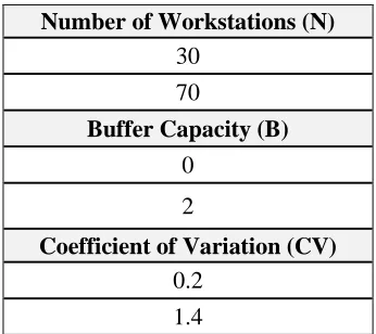
Simulations were performed for each possible combination of the independent variables (see
Table 6). In total 8 (2*2*2) different assembly lines were simulated to test the multiple-bowl
configurations. Then, each of the multiple-bowl configurations were systematically tested in .001
decrements of mean processing time until no statistical improvement on throughput was
achieved, in comparison with the balanced line, according to paired t-test at a 95% confidence
level. The base model was a perfectly balanced line with workstation mean processing time of 1
hour. The multi-bowl configuration with biggest statistically significant improvement on
throughput was selected as the “best multi-bowl configuration” for that condition of line length,
34
Table 6: Independent variable values for multi bowl configurations test
4.4. Preliminary Simulation Model
The unbalanced configurations were tested using the simulation package of Arena Version 14.5.
A preliminary model was designed to simulate the behavior of an unpaced assembly line with
stochastic processing times and buffer capacity between workstation. Based on previous works
(Shaaban & Hudson, 2012), the following assumptions for the model were made:
There are no machine breakdowns
Defective items are not produced.
Single product
No changeover
The time to move work units in and out of the buffers is negligible.
Infinite supply of raw material for the first workstations.
Number of Workstations (N)
30
70
Buffer Capacity (B)
0
2
Coefficient of Variation (CV)
0.2
35
Infinite space for finish good after the last workstation.
Figure 10. Preliminary Simulation Model (3 workstation line)
Figure 10 demonstrated the preliminary model used in Arena to simulate the unpaced assembly
line. The module “Separate 1” allows the simulation of an infinite inventory of raw material for
the first workstation. The module “Seize 1” allows the control of the raw material flow. The
module “Process 1” simulates the workstation 1. The module “Seize 2” allows the simulation of
a buffer between workstation 1 (module Process 1) and workstation 2 (module Process 2), which
release an entity (workpiece) when workstation 2 finished processing. The capacity of the
resource being seized represents the desired buffer capacity between workstations.
4.4.2. Simulation Run Parameters
In order to ensure that what is being observed is as close to normal operating behavior as
possible, a steady-state simulation model was analyzed. A steady-state simulation model has no
natural termination time. In such models, the designer is interested in long term dynamics and
statistics. An example of a steady-state system is an assembly line that operates 24 hours a day,
or an assembly line that always has some WIP at the end of a work day.
The simulation model used in this investigation initiates in an empty and idle state. This means
36
this might be the way things actually start out. However, in a steady-state simulation, initial
conditions are not supposed to matter, and the run is supposed to go on forever.
The simulation initial “atypical” history is called transient-state, as opposed to the simulation
“typical” history that evolves later, which is called the steady-state. The transient-state regiment
is characterized by statistics that vary as a function of time, while steady-state regimen prevails
when statistics stabilize and do not carry over time. In between these two regimes, there is
typically a transition period when the systems approaches the steady-state regimen, a period
characterized by small and generally decreasing variability of the statistics over time. For all
practical purposes, the systems may be considered to be approximately in steady-state during that
transition period (Kelton, Sadowski, & Swets, 2010). In steady-state simulation, only long term
statistics are of interest, but initial systems conditions tend to bias the long term statistics.
Therefore, the statistics were collected after a warm-up period, when the biasing effect of the
initial conditions decayed to insignificant.
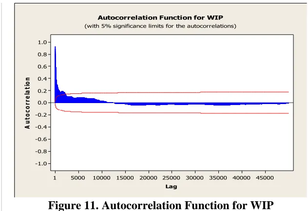
To calculate the necessary warm-up period for the simulation model the method described by
Law (2000) was implemented. A pilot test (with a three workstations balanced line, Normal
distributed mean processing time of 1 hours, coefficient of variation of 0.25, and buffer capacity
of 1unit) was run for 50,000 hours to analyze the behavior of the WIP.
The data of the WIP over time was analyzed in Minitab v.16 and autocorrelation values
calculated. After a period of 2,300 hours autocorrelation values between 0.20 and -0.20 were
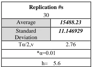
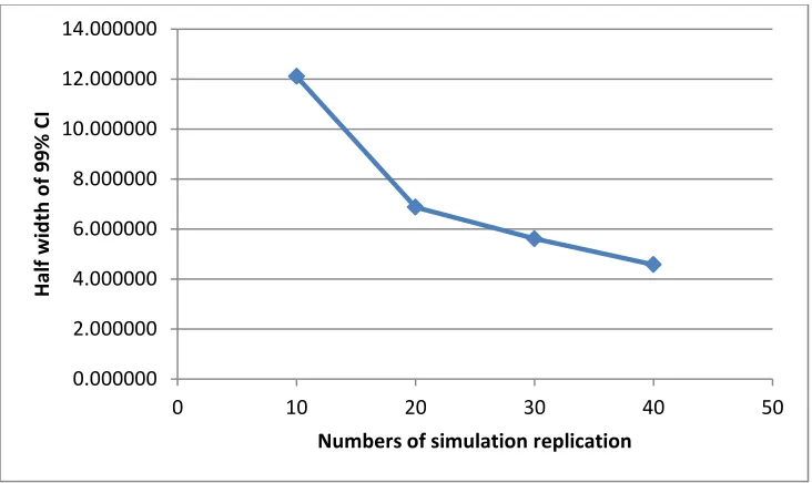
achieved (See Figure 11), which as suggested by McNamara (2011) should ensure steady-state