arXiv:hep-th/9511093v1 14 Nov 1995
UFIFT-HEP-95-29 November 1995
On the origin of three generation
free fermionic superstring models
∗Alon E. Faraggi
† ‡
Department of Physics, University of Florida Gainesville, FL 32611
ABSTRACT
The three generation superstring models in the free fermionic models have had remarkable success in describing the real–world. The most explored models use the NAHE set to obtain three generations and to separate the hidden and observable sectors. It is of course well known that the full NAHE set is not required in order to construct three generation free fermionic models. I argue that all the semi–realistic free fermionic models that have been constructed to date correspond to Z2 ×Z2
orbifolds. Thus, the successes of the semi–realistic free fermionic models, if taken seriously, suggest that the true string vacuum is aZ2×Z2 orbifold with nontrivial
background fields and quantized Wilson lines.
∗ work supported by DE–FG05–86ER–40272.
1. Introduction
The realistic free fermionic superstring models have had remarkable success in accounting for the observed low energy physics [1]. Not only do these models give rise to three chiral generations with the correct quantum numbers under the Standard Model gauge group, but perhaps more impressive is their success in providing plausible explanation to various properties of the observed low energy spectrum, like the stability of the proton [2] and the fermion mass hierarchy [3]. Perhaps the most outstanding success of the realistic free fermionic models is the correct prediction of the top quark mass [4], that was obtained in the context of these models several years prior to the experimental observation of the top quark by the CDF/D0 collaborations.
The successes of the realistic free fermionic superstring models may lead one to speculate that this indeed may be the path that nature has chosen. It should be emphasized that it is not claimed that one of the string models that were constructed to date is the string vacuum that nature has chosen. Indeed, such a claim will require far more elaborate analysis than has been performed to date. However, the remarkable successes of the free fermionic superstring models provide evidence that suggest that the eventually emerging true string vacua will share some of the basic underlying features of the realistic free fermionic models.
Taking this point of view, it is then of extreme importance to try to extract what are the basic underlying features of the realistic free fermionic models. One of the common properties of the realistic free fermionic superstring models is the fact that they all have three chiral generations.
for-mulation in the sense that we can continuously deform the parameters of the com-pactified space and connect between string vacua that in the fermionic formulation would appear as distinct models. Thus, an extremely important task is to try to determine what is the underlying compactification of the realistic free fermionic models.
In this talk I argue that the underlying compactification of all the three gen-eration free fermionic superstring models (that have been constructed to date) is
Z2 ×Z2 orbifold compactification. A very simple realization of this underlying
geometry is achieved with the so called “NAHE” set. However, it is well known that the complete NAHE∗ set is not required for obtaining three generations free fermionic models [8]. I argue that also in the case of non-NAHE models, there is an underlying compactification of a Z2 ×Z2 orbifold. I propose that the
suc-cesses of the realistic free fermionic models, if taken seriously, indicate that the true string vacuum is a Z2 ×Z2 orbifold with nontrivial background fields and
quantized Wilson lines.
2. Three generation models with the NAHE set
In the free fermionic formulation of the heterotic string in four dimensions all the world–sheet degrees of freedom required to cancel the conformal anomaly are represented in terms of free fermions. For the left–movers one has the usual space– time fields Xµ,ψµ, (µ= 0,1,2,3), and in addition the following eighteen real free fermion fields: χI, yI, ωI (I = 1,· · ·,6), transforming as the adjoint representation of SU(2)6
. A model in this construction is defined by a set of boundary condi-tion basis vectors, which are constrained by the string consistency requirements. The basis vectors generate a finite additive group Ξ. The physical states in the Hilbert space, of a given sector αǫΞ, are obtained by acting on the vacuum with bosonic, and fermionic operators. For a periodic complex fermion f, there are two degenerate vacua |+i,|−i , annihilated by the zero modes f0 and f0∗ and with
fermion numbers F(f) = 0,−1, respectively. The physical spectrum is obtained by applying the generalized GSO projections.
The basis vectors of the NAHE set are {1, S, b1, b2, b3} with a choice of
gener-alized GSO projections [11]. The sector S generates N = 4 space–time supersym-metry, which is broken toN = 2 and N = 1 space–time supersymmetry by b1 and
b2, respectively. The gauge group after the NAHE set is SO(10)×E8×SO(6)3.
At the level of the NAHE set, each sector b1,b2 and b3 give rise to 16 spinorial 16
of SO(10). The Neveu-Schwarz sector produces massless states that transform as (5⊕¯5) of SO(10) and as singlets of SO(10)×E8.
The NAHE set divides the internal world–sheet fermions into several groups. The internal 44 right–moving fermionic states are divided in the following way:
¯
ψ1,···,5 are complex and produce the observable SO(10) symmetry; ¯φ1,···,8 are
complex and produce the hidden E8 gauge group; {η¯1,y¯3,···,6}, {η¯2,y¯1,2,ω¯5,6}, {η¯3,ω¯1,···,4} give rise to the three horizontal SO(6) symmetries. The left–moving
{y, ω} states are divided to, {y3,···,6}, {y1,2, ω5,6}, {ω1,···,4}. The left–moving
χ12, χ34, χ56 states carry the supersymmetry charges.
An important consequence of the NAHE set is observed by extending the
SO(10) symmetry to E6. Adding to the NAHE set a vector X with periodic
boundary conditions for the set {ψ¯1,···,5
,η¯1,2,3}, extends the gauge symmetry to
E6×U(1)2×SO(4)3. The sectors (bj;bj+X), (j = 1,2,3) each give eight 27 of
E6. The (N S;N S+X) sector gives in addition to the vector bosons and spin two
states, three copies of scalar representations in 27 + ¯27 ofE6.
In this model the fermionic states which count the multiplets of E6 are the
internal fermions{y, w|y,¯ ω¯}. The vacuum of the sectorsbj contains twelve periodic fermions. Each periodic fermion gives rise to a two dimensional degenerate vacuum
|+iand |−iwith fermion numbers 0 and−1, respectively. After applying the GSO projections, we can write the vacuum of the sector b1 in combinatorial form
+ 2 2
! "
5 1
!
+ 5 3
!
+ 5 5
!#
1 1
!)
(1)
where 4 ={y3y4, y5y6,y¯3y¯4,y¯5y¯6}, 2 ={ψµ, χ12}, 5 = {ψ¯1,···,5}and 1 ={η¯1}. The
combinatorial factor counts the number of |−i in a given state. The two terms in the curly brackets correspond to the two components of a Weyl spinor. The
10 + 1 in the 27 of E6 are obtained from the sector bj +X. The states which count the multiplicities of E6 are the internal fermionic states {y3,···,6|y¯3,···,6}. A
similar result is obtained for the sectors b2 and b3 with {y1,2, ω5,6|y¯1,2,ω¯5,6} and {ω1,···,4|ω¯1,···,4}respectively, which suggests that these twelve states correspond to
a six dimensional compactified orbifold with Euler characteristic equal to 48.
The same model is generated in the orbifold language by moding out anSO(12) lattice by a Z2×Z2 discrete symmetry with standard embedding [9]. The SO(12)
lattice is obtained for special values of the metric and antisymmetric tensor and at a fixed point in compactification space. The metric is the Cartan matrix of
SO(12) and the antisymmetric tensor is given by bij = gij for i > j. The sectors
b1,b2and b3 correspond to the three twisted sectors in the orbifold models and the
Neveu–Schwarz sector corresponds to the untwisted sector.
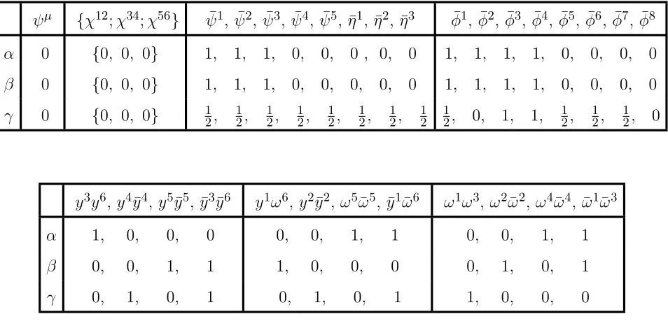
The reduction to three generations is illustrated in table 1. In the realis-tic free fermionic models the vector X is replaced by the vector 2γ in which
{ψ¯1,···,5,η¯1,η¯2,η¯3,φ¯1,···,4} are periodic. This reflects the fact that these models
have (2,0) rather than (2,2) world-sheet supersymmetry. At the level of the NAHE
set we have 48 generations. One half of the generations is projected because of the vector 2γ. Each of the three vectors in table 1 acts nontrivially on the degenerate vacuum of the fermionic states {y, ω|y,¯ ω¯} that are periodic in the sectors b1, b2
and b3 and reduces the combinatorial factor of Eq. (1) by a half. Thus, we obtain
one generation from each sector b1, b2 and b3.
In the previous section we saw how three generation free fermionic models are obtained if the basis contains the full NAHE set,{1, S, b1, b2, b3}. In these models
the connection with theZ2×Z2 orbifold is readily established. The basis vector b3
is replaced with the basis vector ξ1= 1 +b1+b2+b3. The set {1, S, ξ1}generates
a toroidal compactified model withN = 4 supersymmetry and SO(28)×E8 gauge
group. The boundary condition vectors b1 and b2 the correspond to the Z2 ×Z2
orbifold twist. The three sectors b1, b2 and b3 = 1+b1+b2+ξ1 then correspond
to three twisted sectors of the Z2 ×Z2 orbifold model. The reduction to three
generations is achieved by reducing the number of fixed points from each twisted sector to one, by adding three additional boundary condition basis vectors. Each subsequent boundary condition basis vector reduce the number of fixed points from each sector b1, b2 and b3 by a factor of two. At the same time the gauge
group is broken to one of the maximal subgroups ofSO(10). Many other desirable phenomenological properties, like doublet–triplet splitting, can be achieved for appropriate assignment of the boundary conditions in the additional boundary condition basis vectors.
The free fermionic formulation is formulated at a point in the moduli space that may be prefered from a dynamical point of view. The reason being that the free fermionic formulation is formulated near the self–dual point in the com-pactification space. Studies of the effective moduli potential within the context of dynamical supersymmetry breaking by gaugino condensates, indeed suggest that moduli VEVS of the order of the self–dual radius minimize the effective moduli potential [10]. The structure exhibited by the NAHE set is then seen to be very robust in getting three generation models with very desirable phenomenological properties.
perhaps we will be able to guess the correct string compactification, or the correct neighborhood of the true string vacuum.
In the language of the free fermionic models the low energy phenomenological properties are related to the choices of boundary condition basis vectors and gen-eralized GSO phases. We can then ask which choices of basis vectors and GSO phases, in this limited class of models, are necessary to obtain certain desirable phe-nomenological properties. One such phephe-nomenological criteria is the requirement of three chiral generations.
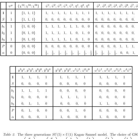
While the NAHE set provides an elegant way for obtaining three chiral gen-erations, it is of course well known that the full NAHE set is not required for constructing three generation free fermionic models. The first published example of such a model was published in Ref. [8]. This model is shown in table 3 (with a slight change of notation). In this model the sectors that may produce chiral generations are the sectors b1, b2 and b3. The degenerate vacuum of the fermionic
zero modes can be represented similar to Eq. (1). The internal fermionic states can also be divided into the same groups as with the NAHE set. Each sector bj then gives rise to 16 generations. This number is then reduced by the choices of boundary conditions in the remaining boundary condition basis vectors. It is easy to see from table 2 that in this model the sector b1 and b2 give rise to one and
two generations respectively. From the table we observe that the degeneracy of the vacuum due to the real fermions in the sector b1 is removed completely, while in
the sectorb2 a double degeneracy remains. The sector b3does not obey the
chiral-ity condition of Ref. [11] and therefore gives rise only to non-chiral matter. The chirality condition of Ref. [11] states that to obtain from a given sector, bj, chiral 16 representation ofSO(10) we need a second vector, bk, with{ψµ,ψ¯1···5}periodic
model the sector b3 produces one 16 and one 16 representation of SO(10).
This model is an example how three generation can be obtained with-out the full NAHE set. Of course, there may exist many other possibilities. For example, as shown in Ref. [8] it is possible to add the vector α with
{y5, ω5, y6, ω6,|y¯5,ω¯5,y¯6,ω¯6,η¯1,φ¯6,···,8} periodic and the remaining boundary
con-ditions antiperiodic to the basis of table 3. With this basis vector, the combination
b1+αprojects the 16 from the sector b3 and reduces the double degeneracy of the
generations from the sector b2. Thus, with basis vector α this model contains one
generation from each sector b1, b2 and b3.
The important question, however, is whether all these three generation models possess some common structure.
The answer, of course, is that all these models are related toZ2×Z2 orbifolds.
The orbifold moding however does not act on a torodially compactified model with
N = 4 space–time supersymmetry and SO(12)×E8×E8 orSO(12)×SO(16)×
SO(16) gauge group, as in the case of the models that contain the full NAHE set. In the non–NAHE models, the sectors ξ1 and ξ2 that produce the spinorial
of SO(16) in the observable and hidden E8s are not present, therefore the space–
time gauge group of the torodially compactified model is SO(44). This gauge symmetry is obtained in the bosonic formulation for appropriate choices of the metric, antisymmetric tensor and Wilson lines [12].
In the Kagan–Samuel model above the basis vectors {1, S} generates a toro-dially compactified model with N = 4 andSO(44) gauge group. The basis vectors
b1 and b2 correspond to the Z2×Z2 orbifold twisting. The third twisted sector
of the orbifold model is still present, and is the combination 1+b1+b2. In this
model the vector ξ2 which generates the spinorial representation of SO(16) in the
adjoint representation of the hidden E8 gauge group is absent. Consequently, the
states from the third twisted sector, 1+b1+b2, are not massless states.
time supersymmetry. The only way to reduce the number of supersymmetry gen-erators that are produced by this basis vector, is by moding by a Z2×Z2 twist.
Therefore, the connection between the three generation free fermionic models and
Z2×Z2 orbifold compactification is in fact expected. By free fermions we confine
ourselves to conformal field theory blocks that are either complex fermions or Ising model operators. Recently, it was found that three generation models can also be obtained if one relaxes this constraint [13]. In the models of Ref. [13], the vectorS is used to generate the space–time supersymmetry. Consequently, in this models, the Z2× Z2 structure is preserved in the supersymmetric sector, while
it is relaxed in the bosonic sector. These models make use of more complicated conformal solutions that do not correspond to free fermions.
4. Conclusion
In this talk, I discussed the correspondence between three generation free fermionic models and orbifold compactification. All the three generation free fermionic models that have been constructed to date correspond to Z2×Z2
orb-ifold compactifications. Other compactifications may be constructed in the free fermionic formulation by using different supersymmetry generators [14] (It is of course possible that these SUSY generators can also lead to three generation mod-els). If the successes of the realistic free fermionic models are to be taken seriously, then they indicate that the true string vacuum is related to a Z2×Z2 orbifold
REFERENCES
1. I. Antoniadis et. al., Phys. Lett. B231 (1989) 65; A.E. Faraggi, D.V.
Nanopoulos and K. Yuan, Nucl. Phys. B335 (1990) 347; I. Antoniadis, G. K. Leontaris and J. Rizos, Phys. Lett. B245 (1990) 161; A.E. Faraggi, Phys. Lett. B278(1992) 131; Nucl. Phys. B387 (1992) 239, hep-th/9208024; J.L. Lopez, D.V. Nanopoulos, and K. Yuan, Nucl. Phys. B399 (1993) 654, hep-th/9203025.
2. A.E. Faraggi, Nucl. Phys. B428 (1994) 111.
3. J.L. Lopez and D.V. Nanopoulos, Nucl. Phys. B338 (1990) 73; Phys. Lett. B251(1990) 73; A.E. Faraggi, Nucl. Phys. B407(1992) 57; A.E. Faraggi and E. Halyo, Nucl. Phys. B416 (1994) 63.
4. A.E. Faraggi, Phys. Lett. B274 (1992) 47.
5. P. Candelas, G.T. Horowitz, A. Strominger and E. Witten, Nucl. Phys. B258
(1985) 46.
6. L. Dixon, J.A. Harvey, C. Vafa and E. Witten, Nucl. Phys. B261 (1985) 678; Nucl. Phys. B274 (1986) 285.
7. H. Kawai, D.C. Lewellen, and S.H.-H. Tye, Nucl. Phys. B288 (1987) 1; I. Antoniadis, C. Bachas, and C. Kounnas, Nucl. Phys. B289 (1987) 87; I. Antoniadis and C. Bachas, Nucl. Phys. B298 (1988) 586.
8. A. Kagan and S. Samuel, Phys. Lett. B284 (1992) 289.
9. A.E. Faraggi, Phys. Lett. B326 (1994) 62.
10. B. de Carlos, J.A. Casas and C. Mu˜noz, Nucl. Phys. B399 (1993) 623.
11. A.E. Faraggi and D.V. Nanopoulos, Phys. Rev. D48 (1993) 3288.
12. K.S. Narain, Phys. Lett. B169 (1986) 41; K.S. Narain, M.H. Sarmadi and E. Witten, Nucl. Phys. B279 (1987) 369.
14. H. Dreiner, J.L. Lopez, D.V. Nanopoulos and D. Reiss, Nucl. Phys. B320
(1989) 401; G. Cleaver, hepth/9505080.
15. L.E. Iba˜nez et al., Nucl. Phys. B301 (1988) 157; L.E. Iba˜nez et al., Phys.
Lett. B191 (1987) 282; A. Font et al., Nucl. Phys. B331 (1990) 421; J.A.
ψµ {χ12;χ34;χ56} ψ¯1, ¯ψ2, ¯ψ3, ¯ψ4, ¯ψ5, ¯η1, ¯η2, ¯η3 φ¯1, ¯φ2, ¯φ3, ¯φ4, ¯φ5, ¯φ6, ¯φ7, ¯φ8
α 0 {0, 0, 0} 1, 1, 1, 0, 0, 0 , 0, 0 1, 1, 1, 1, 0, 0, 0, 0
β 0 {0, 0, 0} 1, 1, 1, 0, 0, 0, 0, 0 1, 1, 1, 1, 0, 0, 0, 0
γ 0 {0, 0, 0} 12, 1 2, 1 2, 1 2, 1 2, 1 2, 1 2, 1 2 1
2, 0, 1, 1, 1 2,
1 2,
1 2, 0
y3
y6
,y4
¯
y4
, y5
¯
y5
, ¯y3
¯
y6
y1
ω6
, y2
¯
y2
, ω5
¯
ω5
, ¯y1
¯
ω6
ω1
ω3
, ω2
¯
ω2
,ω4
¯
ω4
, ¯ω1
¯
ω3
α 1, 0, 0, 0 0, 0, 1, 1 0, 0, 1, 1
β 0, 0, 1, 1 1, 0, 0, 0 0, 1, 0, 1
[image:12.612.69.546.126.364.2]γ 0, 1, 0, 1 0, 1, 0, 1 1, 0, 0, 0
Table 1. A three generations model with the NAHE set. The choice of generalized GSO
co-efficients is: c bj α, β, γ
!
=−c α
1
!
=c α β
!
=−c β
1
!
=c γ
1, α !
=−c γ β
!
=−1
ψµ {χ12;χ34;χ56} ψ¯1, ¯ψ2, ¯ψ3, ¯ψ4, ¯ψ5, ¯η1, ¯η2, ¯η3 φ¯1, ¯φ2, ¯φ3, ¯φ4, ¯φ5, ¯φ6, ¯φ7, ¯φ8
1 1 {1, 1, 1} 1, 1, 1, 1, 1, 1, 1, 1 1, 1, 1, 1, 1, 1, 1, 1
S 1 {1, 1, 1} 0, 0, 0, 0, 0, 0, 0, 0 0, 0, 0, 0, 0, 0, 0, 0
b1 1 {1, 0, 0} 1, 1, 1, 1, 1, 1, 0, 0 0, 0, 0, 0, 0, 0, 0, 0
b2 1 {0, 1, 0} 1, 1, 1, 1, 1, 0, 1, 0 0, 0, 0, 0, 0, 0, 0, 0
b3 1 {0, 1, 0} 1, 1, 1, 1, 1, 0, 1, 0 0, 0, 0, 0, 0, 0, 0, 0
P 0 {0, 0, 0} 0, 0, 0, 0, 0, 0, 0, 0 0, 0, 0, 0, 1, 1, 1, 1
α 0 {0, 0, 0} 12, 1 2, 1 2, 1 2, 1 2, 1 2, 1 2, 1 2 1 2, 1 2, 1 2, 1
2, 0, 0, 1, 1
y3y4,y5y¯5, y6y¯6, ¯y3y¯4 y1y¯6, y2y¯2, ω5ω¯5, ¯ω6ω¯6 ω1ω¯1, ω2ω¯2,ω3ω¯3,ω4ω¯4
1 1, 1, 1, 1 1, 1, 1, 1 1, 1, 1, 1
S 0, 0, 0, 0 0, 0, 0, 0 0, 0, 0, 0
b1 1, 1, 1, 1 0, 0, 0, 0 0, 0, 0, 0
b2 0, 0, 0, 0 1, 1, 1, 1 0, 0, 0, 0
b3 0, 1, 1, 0 0, 0, 0, 0 1, 1, 0, 0
P 0, 1, 0, 0 0, 0, 1, 0 0, 0, 0, 0
[image:13.612.62.536.120.595.2]α 0, 0, 0, 1 1, 0, 0, 0 1, 0, 0, 0
Table 2. The three generations SU(5)×U(1) Kagan–Samuel model. The choice of GSO
phases is: c S
1, bj
!
=−c S P, α
!
=c b1 b2, b3
!
=c b2 b3
!
=−c bj P
!
=−c b1 α
!
= 1
(j=1,2,3) and c b2, b3 α
!
=i, with the others specified by modular invariance and space–