Deductive temporal reasoning with constraints

Deductive Temporal Reasoning with Constraints

Clare Dixon∗_{, Boris Konev}∗_{, Michael Fisher}∗_{, Sherly Nietiadi}∗ Department of Computer Science, University of Liverpool, Liverpool, U.K.

Abstract

When modelling realistic systems, physical constraints on the resources available are often required. For example, we might say that at most N processes can access a particular resource at any moment, exactlyM participants are needed for an agreement, or an agent can be in exactly one

modeat any moment. Such situations are concisely modelled where literals are constrained such that at most N, or exactly M, can hold at any moment in time. In this paper we consider a logic which is a combination of standard propositional linear time temporal logic with cardinality constraints restricting the numbers of literals that can be satisfied at any moment in time. We present the logic and show how to represent a number of case studies using this logic. We propose a tableau-like algorithm for checking the satisfiability of formulae in this logic, provide details of a prototype implementation and present experimental results using the prover.

Keywords: Temporal logic, Constraints, Theorem Proving, Tableau

1. Introduction

Temporal logic allows the concise specification of temporal order. However, if we need to represent cardinality restrictions we have to introduce a large number of formulae to the specifi-cation making it hard to read and understand, and difficult for provers to deal with. In addition, while temporal logic has turned out to be a very useful notation across a number of areas, par-ticularly the specification of concurrent and distributed systems [46, 44, 27], the complexity of many temporal logics is often considered to be too high for practical verification (see for example [11, 8]). Consequently, simple modal logics, finite state automata, or even Boolean satisfiability, are typically used in the verification of such systems. This is because the decision problem for propositional linear temporal logic (PTL) is PSPACE-complete [30] whereas techniques in many of the above areas are much simpler.

So, the question we are concerned with in this work is the following: can we represent and reason about such cardinality restrictions (here we use the term constraints) in a compact and transparent way, retaining the useful descriptive powers of temporal logics, while making the reasoning more efficient in practice? Here we propose and utilise a succinct way of specifying cardinality constraints. We show that if examples are in (or close to) a particular normal form, using this representation of constraints simplifies the reasoning. Additionally, we experiment with an implemented prototype prover for this logic.

To specify the constraints we allow statements stating that less than or equal tok literals, or

exactly k literals from some subset of literals, are true at any moment in time. Note that this approach involves reasoningin the presenceof constraints rather than reasoningaboutthem. Thus, the resulting logic represents a combination of standard temporal logic with (fixed) constraints that restrict the numbers of literals that can be satisfied at any moment in time. This new approach is particularly useful for (for example):

• ensuring that a fixed bound is kept on the number of propositions satisfied at any moment to prevent overload;

∗_{Corresponding author}

• in finite collections of communicating automata, ensuring that no more thankautomata are in a particular state;

• modelling restrictions on resources, for example at mostkvehicles are available or there are at mostkseats available;

• modelling the necessity to elect exactly kfromnparticipants.

Motivating Example. Consider a fixed number,n, of robots that can eachwork,restorrecharge. We assume that there are onlyk < nrecharging points and onlyj < nworkstations. Let:

• worki represent the fact that robotiis working; • resti represent the fact that robotiis resting; and • rechargei represent the fact that robot iis recharging.

Now, we typically want to specify that exactlyj of thenrobots are working at any one time. In the syntax given later, such a logic might be defined as TLC(W=j_,R6k_{), where}

W=j _{= {work}

1, . . . , workn}=j R6k _{= {recharge}

1, . . . , rechargen}6k

This represents the logic with the constraints that exactlyjrobots must work at any moment and at mostkcan recharge at any moment.

This paper extends preliminary material from our earlier paper [19]. The contributions of the paper are: to define and analyse a logic which combines both temporal logic and constraints; to show how a number of case studies can be elegantly modelled using this logic; to provide a tableau-like satisfiability algorithm for formulae in this logic giving proofs of correctness; to provide algorithms for a prototype implementation of this; and give experimental results comparing the implementation with other temporal provers.

The paper is organised as follows. Section 2 gives the syntax and semantics of the constrained temporal logic, together with a normal form for this logic. In Section 3 we provide a number of case studies and show how they are specified in this logic. In Section 4 we provide an algorithm for checking satisfiability of this logic and consider its complexity. In Section 5 we give details of an implementation of the satisfiability checker for this logic and experimental details comparing this implementation to other tableau reasoners for propositional linear time temporal logic. Finally, in Section 6, we provide concluding remarks and discuss both related and future work.

2. A Constrained Temporal Logic

Temporal Logic with Cardinality Constraints (TLC) [19] is PTL with some additional con-straints, which restrict the numbers of literals that can be satisfied at any moment in time. TLC is parameterised by (not necessarily disjoint) sets C∝m _{where ∝∈ {=,}

6} andm ∈_N. The for-mulae of TLC(C∝1m1

1 , C

∝2m2

2 ,· · ·) are constructed under the restriction that, depending on ∝i,

exactly mi literals from every setCi are true in every state (∝i is =) or less than or equal tomi

literals from every setCiare true in every state (∝i is6). For example, consider TLC(C1=2, C6 1 2 ),

whereC=2

1 ={p, q, r}=2andC6 1

2 ={x, y, z}6

1_{. Then, at any moment of time, exactly two ofp, q,}

or rare true, and less than or equal to one ofx, y, orz is true. In addition to these constraints, there exists a set of propositions,A, which are standard, unconstrained propositions. Note that, the ‘less than’ constraintC<m _{can be expressed asC}6m−1 _{and the ‘more than or equal to’}

con-straintC>m_{can be expressed as ¯C}6n−m_{, wherenis the number of literals inCand by definition}

¯

C = {x¯ | x∈ C}, ¯p = ¬p and ¬p = p. Note that by using both C6m _{and C}>m _{(encoded as}

¯

C6n−m_{) we could also obtain C}=m_{. However we choose not to do this, as we aim for a clear}

and intuitive way of expressing constraints and this appears to obscure the meaning. Further, the constraintC=1 _{seems to be common in applications (see Section 3) which gives additional weight}

for theC=m_{construct to be primitive.}

We note that we can express the information in our constrained sets as temporal formulae. For example given the constraint C₁=2 ={p, q, r}=2 _{above, this can be represented by the following}

temporal formula.

2.1. TLC Syntax

A constraintC∝imi

i is a tuple (Ci,∝i, mi), whereCiis a set of literals with a cardinality

restric-tion∝i mi, such that ∝i∈ {=,6} and mi ∈N. For TLC, the future-time temporal connectives

we use include ‘ g’ (in the next moment) and ‘U’ (until). Formally, TLC(C∝1m1

1 ,· · ·, Cn∝nmn)

formulae are constructed from the following elements:

• a set, Props={p|p∈C∝imi

i } ∪ {p| ¬p∈ C

∝imi

i } ∪ A of propositional symbols (where

1₆i₆nandAare termed ‘unconstrained’ propositions);

• propositional connectives, true,¬,∧; and

• temporal connectives, g,and U. We also write TLC(C), where C={C∝1m1

1 ,· · · , Cn∝nmn}.

The set of well-formed formulae (_wff) of TLC, is defined as the smallest set satisfying the following:

• any elements of Propsandtrueare in _wff;

• ifϕandψare in _wff, then so are¬ϕ, ϕ∧ψ, gϕ, ϕU ψ.

A literal is defined as either a proposition symbol or the negation of a proposition symbol. We (ambiguously) assume that the negation of¬pisp.

2.2. TLC Semantics

First we define the satisfiability of a constraint. The notationL |=P L ϕdenotes the truth of

propositional logic formulaϕwith respect to a set of propositionsL. L |=P Lpiffp∈ L wherep∈

Propsand the semantics of the operators¬, ∧is as usual. LetLbe a set of propositions, C∝m_a

constraint and

Eval(L, C∝m) ={p|p∈ Landp∈C} ∪ {¬p|p6∈ L and¬p∈C}

then

L |=P LC=m iff |Eval(L, C=m)|=m, L |=P LC6m iff |Eval(L, C6m)|6m.

Note that the operator|=P Lis only defined for formulae from propositional logic (not from

tempo-ral logic). A setCof constraints issatisfiable(|=P L C) if, and only if, there is a set of propositions L, such that, for eachC∝imi

i ∈ C (i∈N),L |=P LCi∝imi.

A model for TLC(C) formulae can be characterised as a sequence of states, σ, of the form σ = s0, s1, s2, s3, . . ., where each state si is a set of propositional symbols representing those

propositions, which are satisfied at the ith _{moment in time. Every s}

i should satisfy the set of

constraints,C, i.e., for allsi we havesi |=P LC (wheresi is a set of propositions).

The notation (σ, i)|=ϕdenotes the truth of formula ϕ in the modelσ at the state of index i∈_Nand is defined as follows.

(σ, i)|= true

(σ, i)|= p iffp∈si wherep∈Props

(σ, i)|= ¬ϕ iff it is not the case that (σ, i)|=ϕ (σ, i)|= ϕ∧ψ iff (σ, i)|=ϕand (σ, i)|=ψ (σ, i)|= gϕ iff (σ, i+ 1)|=ϕ

(σ, i)|= ϕUψ iff∃k∈N. k>iand (σ, k)|=ψand

∀j∈N, ifi6j < kthen (σ, j)|=ϕ

Note we can obtainfalseand the other Boolean operators via the usual equivalences and we define ‘ ’ (always in the future), ‘

♦

’ (sometime in the future) and ‘W’ (unless or weak until) operators as follows.

♦

ϕ ≡ trueUϕ ϕ ≡ ¬

♦

¬ϕ

For any formulaϕ, modelσ, and state indexi∈N, either (σ, i)|=ϕholds or (σ, i)|=ϕdoes not

hold, denoted by (σ, i)6|=ϕ. If there is someσsuch that (σ,0)|=ϕ, thenϕis said to besatisfiable. If (σ,0)|=ϕfor all models,σ, thenϕis said to bevalid and is written|=ϕ. A setN of formulae issatisfiable in the modelσat the state of indexi∈Nif, and only if, for allϕ∈ N,(σ, i)|=ϕ.

A formula of the form

♦

ϕ or ψUϕ is called an eventuality. A formula of the form gϕ is called anext-time formula.

2.3. Normal Form

It is often convenient to operate on formulae in a normal form. Separated Normal Form (SNF) was first introduced for PTL in [26] (see also [28]); the normal form for TLC extends one from [28] with ideas from [16]. To assist in the definition of the normal form we introduce a further (nullary) connective ‘start’ that holds only at the beginning of time, i.e.,

(σ, i)|=start iff i= 0.

This allows the general form of the (temporal clauses of the) normal form to be implications. In the following, small Latin letters, ki, lj, m represent literals in the language Propswhere

i, j_>0. Note, on the left hand side, ifi= 0 the empty conjunction represents true whereas, on the right hand side, ifj= 0 the empty disjunction represents false. A normal form for TLC is of the form

^

h

Xh

whereh_>1 and eachXh is aninitial,step, or sometime clause (respectively) as follows:

start ⇒ _

j

lj (initial)

^

i

ki⇒ g

_

j

lj (step)

true⇒

♦

m (sometime)

Sometime clauses defined above are also known asunconditional sometime clauses. SNF defined in [28] allows forconditional sometime clauses—expressions of the form

^

i

ki⇒

♦

m .

However, it was shown in [16] that any PTL formula can be translated into SNF with only unconditional sometime clauses. We can rewrite a conditional sometime clause of the above form into an unconditional one, of the form we require here, using a new propositional variable wm.

Informally, the new proposition wm denotes waiting for m. The resulting clauses replacing the

conditional eventuality are as follows.

true ⇒

♦

¬wm

start ⇒ (W

i¬ki∨m∨wm) true ⇒ g(W

i¬ki∨m∨wm)

wm ⇒ g(m∨wm)

Theorem 1 of [16] shows that a set of clauses with the conditional sometime clauses replaced by the unconditional sometime clause and three additional clauses above preserves satisfiability and Lemma 1 of [16] shows this involves a linear increase in the size of the problem relating to the number of eventualities occurring.

Since the constraints do not affect the normal form, we obtain the following theorem as a corollary of [16].

When specifying the behaviour of systems, it is sometime convenient to consider ‘traditional’ clauses of the form

_

j

lj (global)

Every global clause can, if necessary, be represented as a combination of an initial and a step clause:

start ⇒_ j

lj and true⇒ g

_

j

lj

We will use global clauses in Section 3.

Transformation into the normal form may introduce new (unconstrained) propositions; how-ever, as we will see in Section 3, many temporal formulae stemming from realistic specifications are already in the normal form, or very close to the normal form and require few extra variables for the translation (for other examples, also see [24]).

2.4. Encoding of Constraints

In the case of PTL the addition of constraints does not extend the logic, i.e. we can rewrite any constraintC∝kinto the syntax of PTL. However, our representation of constraints is succinct and allows the prover to make use of this information in a global way. To compare with other provers for PTL we must add formulae that represent these constraints. We use a direct encoding of constraints, which does not introduce extra propositions. ForS being a set of literals andk∈N

we define

pos(S, k) = ^

U⊆S

|U|=|S|+1−k

_

li∈U

li

and

neg(S, k) = ^

U⊆S

|U|=k+1

_

li∈U ¬li

For example, pos({p, q, r},2) = (p∨q)∧(p∨r)∧(q∨r) and neg({p, q, r},2) = ¬p∨ ¬q∨ ¬r. Intuitively,neg(S, k) denotes that for a set of literalsS, to make at mostk true, for every subset of sizek+ 1 at least one of these must be false. Similarly,pos(S, k) denotes that for a set of literals S, to make at most|S| −k false, for every subset of size|S|+ 1−k at least one of these must be true.

Lemma 2 ([53]). Given a set of propositionsL,L |=P L C=k if, and only if, L |=P Lpos(C, k)∧

neg(C, k)andL |=P LC6k if, and only if, L |=P Lneg(C, k).

To generate PTL formulae equivalent to the constraints, then:

• for a constraint of the formC=k we construct (pos(C, k))∧ (neg(C, k));

• for a constraint of the formC6k _{we construct (neg(C, k)).}

For a constraint of the form C6k_{, such a direct encoding contains} n k+1

clauses, which fork =

dn/2e −1 reaches O2n_/p

n/2clauses [53].

We note that other translations are possible. For example we can use the fact that an n-bit counter can represent 2n _{different values. If we required exactly one constraints (C}=1_{) we could}

represent a constraint of the form{p1, p2, p3, p4}=1 using just two propositional variablest01, t02 by

adding the following formulae.

(p1 ⇔ (t01∧t02))

(p2 ⇔ (t01∧ ¬t02))

(p3 ⇔ (¬t01∧t02))

(p4 ⇔ (¬t01∧ ¬t02))

3. Case Studies

Next we consider several case studies and show how they can be specified in TLC. For ease of presentation some of the formulae presented are not strictly in SNF but can be transformed into SNF using simple equivalences. The case studies here are necessarily simplified and are included purely to exemplify the approach; clearly much larger examples can be constructed along similar lines.

3.1. Five-A-Side Football

Consider a team of football playing agents. This could be either a team involving human players or a RoboCup team. The rules say that at most 5 players (i.e. a “five-a-side” game) in the team can be on the field of play at any time. However, other players can be off the field of play, either resting or injured.

Let us begin to model such a scenario using temporal logic. We will describe the current activity of a particular player,i, using the propositionsplayingi,restingi, andinjuredi. Thus:

• playingi represents the fact that player iis actually playing;

• restingi represents the fact that player iis resting; and

• injuredi represents the fact that playeriis injured.

Let us assume, for simplicity that our team has 6 players; to begin with, one is just resting:

start ⇒ playing1 ∧playing2 ∧ playing3 ∧ playing4 ∧ playing5 ∧resting6

We can describe the possible dynamic behaviours, for eachi, as follows.

• when playing, a player can either continue, stop to rest, or become injured: (playing_i⇒ g(playing_i∨resting_i∨injured_i))

• when resting, a player can either continue resting, or return to playing: (restingi ⇒ g(playingi ∨ restingi))

• once injured, a player remains injured:

(injuredi ⇒ ginjuredi)

We might also want to add some formulae describing details of the particular scenario, for example we might want to state that any player resting will eventually get to play:

(restingi ⇒

♦

playingi)

Whilst the above formula is not part of the TLC normal form syntax it can be rewritten into the following equi-satisfiable formulae (see Theorem 1).

(true ⇒

♦

¬wplayingi)

(start ⇒ ¬restingi∨playingi ∨wplayingi) (true ⇒ g(¬restingi∨playingi ∨wplayingi)) (wplayingi ⇒ g(playingi ∨wplayingi))

Of course there are a number of structural constraints that we must also describe for this scenario concerning the relationships between these propositions. For example, we must specify that there are at most 5 players playing at any moment. We do this by describing the constraint:

P65 _{= {playing}

1,playing2,playing3, playing4,playing5,playing6 }65

Another obvious constraint is that each player can only be playing, resting or injured. So, for each player,i, we would describe this constraint as

Mi=1 = {playingi,restingi,injuredi }=1

TLC(P65_,M=1

1 ,M=12 ,M=13 ,M=14 ,M=15 , M=16 )

This provides us with a logic in which the above structural constraints are implicitly enforced at every moment in time and avoids the need to explicitly encode these as temporal formulae.

3.1.1. Viable Teams

Once we have this scenario we can embellish it in many ways. One is to consider not just the rules of the game (i.e. that at most 5 players can be playing at any time) but the viability of the team itself. For example, what if only 2 players are actually playing? Or even 1? Very likely the team will lose quickly. So, we might add another constraint to ensure that the team is always viable, for example:

V63 =

resting1, resting2,resting3,resting4,resting5,resting6,

injured1,injured2, injured3,injured4,injured5,injured6 63

This ensures that at most 3 players are resting or injured, and so at least 3 players are actually playing. AddingV63_{to our TLC definition ensures that only viable teams are described.}

3.1.2. Goalkeeper

Another embellishment might be to add a ‘goalkeeper’. This is a player who is designated to defend the goal. Let us add another set of propositions, goalkeeperi, which is true if the playeri is the goalkeeper. Clearly, the goalkeeper must be playing:

(goalkeeperi ⇒ playingi)

But the role of being a goalkeeper can move between players. So, if a player is not a goalkeeper now they will eventually take on this role:

(¬goalkeeperi ⇒

♦

goalkeeperi)

The above needs to be rewritten into SNF similarly to that previously described. Finally, and most obviously, we need structural constraints concerning the goalkeeper proposition. In particular, at most one player can be the goalkeeper at any moment. (Note that we might not have any

goalkeeper!) So, we add the constraint setG61_:

{goalkeeper1,goalkeeper2, goalkeeper3,goalkeeper4,goalkeeper5,goalkeeper6}61

3.1.3. Properties

There are many potential properties to prove. For example, we might show that if all the players eventually become injured then the team is unviable. Thus, if we add

♦

(injured1 ∧ injured2 ∧ injured3 ∧ injured4 ∧ injured5 ∧ injured6)

then the whole set of formulae should be unsatisfiable.

Another property we might show is that, as long as there are no injuries, then eventually every player will take a turn as the goalkeeper. Thus the specification so far, together with

V

i¬injuredi, should imply

♦

goalkeeper1 ∧

♦

goalkeeper2 ∧

♦

goalkeeper3∧

♦

goalkeeper4 ∧

♦

goalkeeper5 ∧

♦

goalkeeper6

3.2. Cache Coherence Protocol

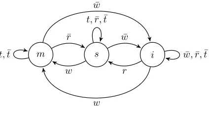
We next consider using our logic to specify a simple cache coherence protocol with a finite number of processes. Each processor has its own private cache memory which holds local copies of the main memory blocks. Cache coherence protocols aim to ensure the consistency of the cache for different processors. Abstracting away from low level details we can describe such protocols as a family of identical finite state systems together with a primitive form of communication.

s

m i

t,¯t

¯ r

¯ w

t,r,¯ ¯t ¯ w

w

¯ w,¯r,t¯ r

[image:8.612.197.409.65.180.2]

w

Figure 1: Finite state machine for the MSI protocol.

representation of this protocol has been given in [45]. At any moment one process is active and, depending on its state, may carry out a readr, a writewor a local transitiont. The action is then broadcast to all the other processes, which carry out a reaction to what has happened (denoted ¯

r, ¯wor ¯trespectively). This is shown in the transition system in Figure 1.

τ(i, w) =m τ(s, w) =m τ(m,w) =¯ i τ(i,w) =¯ i τ(s,w) =¯ i τ(m,r) =¯ s τ(i, r) =s τ(s,r) =¯ s τ(m, t) =m τ(i,¯r) =i τ(s, t) =s τ(m,t) =¯ m τ(i,¯t) =i τ(s,¯t) =s

Initially all processes are in the stateiand we should show that

• it is never possible that one process is in statemwhile another is in states(non co-occurrence of statessandm);

• it is always the case that at most one process can be in statem. We can represent this for a finite number of processes where

aj means that processj is active;

mj means that processj is in the statem;

sj means that processj is in the states;

ij means that processj is in the statei.

Rather than representingw,randtfor each process we will allow one for the system where if that process is not active it means that the process is reacting, i.e. carrying out a ¯w, ¯r, or ¯ttransition. There are a number of constrained sets. Givennprocesses, for each process j we have

S=1

j ={mj, sj, ij}=1

To make exactly one process active at any moment we have

P=1_={a

1, a2, . . . an}=1

and to ensure only one ofw,r andtholds we have

T=1_{={w, r, t}}=1_.

Thus for n processes we have TLC(S=1 1 , . . . ,S

=1 n ,P

=1_,T=1_{). When a processor is active the}

transitions can be formalised as follows.

((ii∧ai∧w) ⇒ gmi)

((ii∧ai∧r) ⇒ gsi)

((si∧ai∧w) ⇒ gmi)

((si∧ai∧t) ⇒ gsi)

When the processor isnot active the transitions can be formalised as follows.

((ii∧ ¬ai∧w) ⇒ gii)

((ii∧ ¬ai∧r) ⇒ gii)

((ii∧ ¬ai∧t) ⇒ gii)

((si∧ ¬ai∧w) ⇒ gii)

((si∧ ¬ai∧r) ⇒ gsi)

((si∧ ¬ai∧t) ⇒ gsi)

((mi∧ ¬ai∧w) ⇒ gii)

((mi∧ ¬ai∧r) ⇒ gsi)

((mi∧ ¬ai∧t) ⇒ gmi)

The transitions that can be taken when a processor is active are as follows.

((ii∧ai) ⇒ (w∨r))

((si∧ai) ⇒ (w∨t))

((mi∧ai) ⇒ t)

The negation of the two required properties for 6 processes are given below, i.e. conjoining the following with the specification should be unsatisfiable

• non co-occurrence fors andm:

♦

((m1∧s2)∨(m1∧s3)∨(m1∧s4)∨(m1∧s5)∨(m1∧s6)∨(m2∧s1)∨(m2∧s3)∨(m2∧

s4)∨(m2∧s5)∨(m2∧s6)∨(m3∧s1)∨(m3∧s2)∨(m3∧s4)∨(m3∧s5)∨(m3∧s6)∨(m4∧

s1)∨(m4∧s2)∨(m4∧s3)∨(m4∧s5)∨(m4∧s6)∨(m5∧s1)∨(m5∧s2)∨(m5∧s3)∨(m5∧

s4)∨(m5∧s6)∨(m6∧s1)∨(m6∧s2)∨(m6∧s3)∨(m6∧s4)∨(m6∧s5)); • at most one process can be in state m:

♦

((m1∧m2)∨(m1∧m3)∨(m1∧m4)∨(m1∧m5)∨(m1∧m6)∨(m2∧m3)∨(m2∧m4)∨(m2∧

m5)∨(m2∧m6)∨(m3∧m4)∨(m3∧m5)∨(m3∧m6)∨(m4∧m5)∨(m4∧m6)∨(m5∧m6)).

3.3. Petri Nets

Consider now k-safe Petri Nets (see for example [22]), which are used to model systems with limited resources. In k-safe Nets, every ‘place’ may contain at most k tokens. This restriction allows us to represent k-safe Petri Nets, for a fixed value of k, in propositional temporal logic. Encoding places as propositions (propositionpj_i is true if, and only if, placePicontainsj tokens),

given a k-safe Petri Net N, one can construct a PTL formula φN of the size polynomial in the size ofN, such that models ofφN correspond to infinite trajectories ofN.

A Net is a tupleN = (P,T,F, M0) whereP is a set of places, T a set of transitions,F is the

flow relation andM0is the initial marking such that P = {P1, P2, . . . Pn}; T = {x1, x2, . . . xm}; F ⊆ (P × T)∪(T × P);

andM0:P →N. Generally, a mappingM :P →Nis called amarking ofN. A transitionx∈ T

isenabled atM if for everyP such that (P, x)∈ F we haveM(P)6= 0. For markingsM,M0 we writeM −→M0if, and only if, some transitionx∈ T is enabled atM and for every placeP ∈ P

we have

M0(P) =M(P) +F(x, P)−F(P, x),

where F(x, y) is 1 if (x, y)∈ F and 0 otherwise. We say that marking M0 is reachable in N if M0 −→∗ M0, where the relation −→∗ is the reflexive transitive closure of −→. Thereachability problem is to determine given a NetN and a markingM whetherM0 _{is reachable inN.}

that the place contains one or more tokens. Similarlyxj denotes both a transition in the Petri

Net and a proposition representing that transitionxj is fired. Firstly the following constraint, for

eachxi∈ T, states that exactly one transition fires at any moment in time.

{x1, . . . xm}=1

For each Pi ∈ P exactly one of the propositions representing the number of tokens in this place

can be true.

{p0_i, . . . pk_i}=1

We usePi to show when there are tokens in a place. ForPi ∈ P

((p1_i ∨. . . pk_i)⇔Pi)

For each (Pj, xi)∈ F the pre-condition of transitions is represented as follows.

(xi⇒Pj)

For each (Pj, xi)∈ F the effect of each transition is represented as follows for each 16h6k

((ph_j ∧xi)⇒ g(phj−1))

Recall that fork-safe Petri Nets and (xi, Pj)∈ F it is not possible that a transitionxi fires when

place Pj already containsk tokens. Thus, for each (xi, Pj)∈ F the effect of each transition can

be represented as follows for each 0₆h < k

((ph_j ∧xi)⇒ g(phj+1)).

Additionally we must add frame conditions so that the number of tokens in places unrelated to the firing transition remain the same for eachPj ∈ P, for each 06h6k.

((ph j ∧

^

(Pj,xi)∈F

¬xi∧

^

(xi,Pj)∈F

¬xi) ⇒ gphj)

((¬ph_j ∧ ^ (Pj,xi)∈F

¬xi∧

^

(xi,Pj)∈F

¬xi) ⇒ g¬phj)

For example, consider the 1-safe Petri Net (similar to one in [49]), given in Fig. 2, representing the dining philosophers problem [36] for the case of four philosophers. This problem relates to providing processes with concurrent access to a limited number of resources. Here as there is only at most one token in each place we do not introduce the propositions (pj_i) above but let the propositions representing place names (eg Fork1) denote the presence of a token. This Petri Net

can be represented as the conjunction of transition representations

(x1⇒E1) Pre-condition for transitionx1

(x1⇒ g(¬E1∧Fork1∧Fork4∧T1)) Effect of transitionx1

(y1⇒Fork1∧Fork4∧T1) Pre-condition for transitiony1

(y1⇒ g(¬Fork1∧ ¬Fork4∧ ¬T1∧E1)) Effect of transitionx1

. . .(similarly for other transitions)

frame conditions

(Fork1∧ ¬x1∧ ¬x2∧ ¬y1∧ ¬y2⇒ gFork1) Fork1 can only change due to

(¬Fork1∧ ¬x1∧ ¬x2∧ ¬y1∧ ¬y2⇒ g¬Fork1) transitionx1, x2,y1 andy2

. . .(similarly for other places)

and the constraint

{x1, . . . , x4, y1, . . . , y4}=1,

Fork1 Fork2

Fork3

Fork4

E1

T1

y1 x1

E2

T2

y2

x2

E3

T3

y3

x3

E4 T4

y4

[image:11.612.157.448.67.355.2]

x4

Figure 2: Four dining philosophers Petri Net.

constraint means that no other transition can be taken at the same same. The effects are (in the next moment in time) to remove the tokens from places Fork1, Fork4 and T1 and for a token to

be put at E1so philosopher one can eat. Note that due to the well known frame problem we must

explicitly state that the tokens remain in all other places not affected by the selected transition. Reachability in such Nets, for example the reachability of the state E4, corresponds to the

satisfiability of

♦

E4 from an initial state. Since the reachability problem (as well as many other

interesting problems) already for 1-safe Nets is PSPACE-complete [22], such a translation is opti-mal.

We can then use cardinality constraints to impose place invariants: for a subset of places in a Petri Net, the total number of tokens in places from this subset remains constant. Such invariants are used, for example, in the verification of distributed protocols with Petri Nets [42, 43]. Note that imposing such extra restrictions actually makes the complexity of reasoninglower.

3.4. Other Examples

Other examples that have commonly been specified using temporal logics that may benefit from the use of constraints are systems such as the modelling of train movement, see for example [25, 23, 48]. Typical constraints here, for example, require that each station can be occupied by at mostmtrains, each section of the track can contain at most one train, the signals cannot be red and green at the same time, etc. Similarly the specification of lift controllers for example [3, 59] exhibit a number of constraints such as the lift may be at exactly one floor at any moment etc.

we formalise the algorithm for a swarm of foraging robots using a number of transition systems for each robot and the food it is collecting. As well as the constraints that each robot can be in exactly one mode at any moment there are additional constraints that synchronise the transition systems for the food with those for the robots.

4. Satisfiability for TLC

Next we provide an algorithm for checking satisfiability of TLC formulae and also give the upper complexity bound on satisfiability of TLC by the explicit construction of a directed graph known as abehaviour graph.

4.1. Behaviour Graphs

The notion of a behaviour graph for a set of temporal clauses was introduced in [28] and adapted to the unconditional sometime clauses in [16]. It is a directed graph for a set of temporal clauses such that (after reductions) any infinite path through the graph is a model for the set of temporal clauses. Satisfiability of TLC formulae can be checked by being able to construct a non-empty graph. In what follows, we estimate the size of the graph and time needed both for its construction and for checking satisfiability.

Definition 3. (Behaviour Graph/Reduced Behaviour Graph) Given a formula ϕ in the normal form over a set of (both constrained, C, and unconstrained) literals Props, we construct a finite directed graph G as follows. The nodes I of G are interpretations (subsets) of Props, satisfying the required constraints, i.e.I|=P LC.

A node,I, is designated an initial node ofGifI|=P L

_

i

li for every initial clausestart ⇒

_

i

li

of the given temporal formula. For each node, I, we construct an edge in Gto a node I0 if, and only if, the following condition is satisfied:

• For every step rule, ^ i

ki⇒ g

_

j

lj, ifI|=P L

^

i

k thenI0|=P L

_

j

lj.

The behaviour graph,H, ofϕis the maximal subgraph ofGgiven by the set of all nodes reachable from initial nodes. The reduced behaviour graph,HR, ofϕis a graph obtained from the behaviour graph ofϕby repeated deletion of nodes I where

a) I does not have a successor; or

b) for some sometime clausetrue⇒

♦

mwithin ϕ, there is no path from I to a node J where

m is true, that is,J |=P L m.

Theorem 4. A TLC formula in the normal formϕis satisfied if, and only if, its reduced behaviour graph is non-empty.

Proof. The definition of a TLC behaviour graph given above differs from the behaviour graph for PTL, defined in [16], in that we never construct nodes that do not satisfy the set of constraints. Since the expressive power of PTL and TLC is the same, as shown in Lemma 2, this restriction can be imposed by encoding the constraint as a PTL formula. Letψbe a propositional logic formula

equivalentto the constraintsC, i.e. for anyI,I|=P LC if, and only if,I|=P L ψ. Translating ψ

into temporal clauses will result in a number of initial and step clauses. In terms of the behaviour graph in [16] by construction every initial node must satisfy the initial clauses derived from ψ and every non-initial node must satisfy the step clauses derived from ψ. Hence we would never construct an initial node that does not not satisfyψ, further we would never construct an edge to a node not satisfyingψ. That is, nodes not satisfyingψwould be unreachable and thus could not

form part of the behaviour graph.

the satisfiability problem for TLC is also PSPACE-complete. Notice further that if we restrict our consideration to formulae in Separated Normal Form, the size of the TLC behaviour graph is exponential in the number of unconstrained propositions and only polynomial in the number of constrained propositions (see Theorem 5).

Theorem 5. Satisfiability of aT LC(C∝1m1

1 , . . .Cn∝nmn)formulaϕin Separated Normal Form can be decided in time

O

|ϕ| ×|C∝1m1

1 |

m1_{× · · · × |C}∝nmn

n |

mn_×2|A| 3

where|ϕ| is the length ofϕ,|C∝imi

i |is the size of the set C

∝imi

i of constrained literals, and|A| is the size of the set Aof unconstrained propositions occurring inϕ.

Proof. There existO(|C∝1m1_|m1_{×· · ·×|C}∝nmn

n |mn×2|A|) different interpretations of propositions

fromProps; moreover, they can all be enumerated in timeO(|C∝1m1_|m1_{× · · · × |C}∝nmn

n |mn×2|A|).

LetN be the number of such different interpretations of propositions fromProps. The behaviour graphGforφcan be constructed inO(N2_{) time.}

To reduce the behaviour graph we do the following. A node without successors can be found in O(N2) time. To find all nodes satisfying condition b), for every eventualitytrue⇒

♦

mwe first mark all nodes containingmand then work backwards to mark all nodes with a path to a marked node. Every unmarked node satisfies conditionb). This can be done in O(|φ| ×N2) time. (The

|φ| factor comes from the necessity to check this condition for every eventuality true ⇒

♦

m.) This process should be repeated until there is no change. Clearly, the maximal number of nodes to delete isN and thus the process can be repeated at most N times.

Overall, the complexity of reducing the behaviour graph, as well as the complexity of the entire procedure, isO(|φ| ×N3_).

Notice that the TLC formulae stemming from our case studies are all in, or close to, the normal form. In practice, this result suggests that, by exploiting cardinality constraints in TLC, we can achive a better performance on relevant problems than algorithms that have no built in facilities to handle such constraints.

4.2. Incremental Algorithm

Based on Theorem 4 one can provide an algorithm checking the satisfiability of TLC formulae. A straightforward approach is to construct the graphGrepresenting all possible interpretations of Propsthat satisfy the constraints, and then ‘carve’ the behaviour graphH fromG. However, such a procedure might consider some nodes that are actually unreachable from the initial nodes and, thus, carry out excess work. Instead, in Algorithm 1, we present an incremental, tableaux-like algorithm, which avoids building these unnecessary nodes.

Let Assignments(ϕ,C) be a function which, when given a formula ϕ and a set of constraints

C, returns the set of all interpretations within the languageProps that both satisfy C and make ϕtrue. Clearly,Assignments(ϕ,{C∝1m1

1 , . . . , C∝n mn

n }) can be computed deterministically in time

O(int) whereint= (|C∝1m1_|m1_{× · · · × |C}∝nmn

n |mn×2|A|) returning at mostO(int) interpretations

for anyϕ.

Example. IfProps={p, q, r, s}thenAssignments(p∨q,{{p, q, r, s}=1_{}) will return two}

interpreta-tions (where proposiinterpreta-tions not explicitly mentioned are assumed to be false): {p}and{q}; whereas Assignments(p∨q,{{p, q}=1_{,{q, r, s}}=2_{}) will return three: {p, r, s},{q, r}, and{q, s} .}

We useAssignments(ϕ,C) to construct nodes of the behaviour graphH for a formulaϕ incremen-tally (see Algorithm 1ConstructBehaviourGraph(ϕ,C)). Notice that the size of graphH is still worst-case quadratic inint.

Algorithm 1ConstructBehaviourGraph(ϕ,C)

1: Letψ=V

{Rj|start ⇒Rj is an initial clause in ϕ} 2: forallI inAssignments(ψ,C)do

3: Add an unmarked node I toH

4: end for

5: while Not all nodes inH are markeddo 6: Pick an unmarked nodeI and markI

7: Letχ=V

{Rk|Lk⇒ gRk is a step clause inϕs.t. I|=P LLk} 8: forallJ inAssignments(χ,C)do

9: if J is not already inH then 10: Add an unmarked node J to H

11: end if

12: Add an edge (I, J) toH

13: end for 14: end while

Algorithm 2EventualityDelete(H, m)

1: LetBm={nodesI∈H |I|=P L¬m} 2: repeat

3: forall nodesI inBmdo

4: if (I, J) inH andJ 6∈Bmthen 5: Bm=Bm− {I}

6: end if

7: end for

8: untilBmdoes not change 9: Delete(Bm)

Algorithm 3ReducedBehaviourGraph(ϕ,C)

1: H = ConstructBehaviourGraph(ϕ,C)

2: repeat

3: if there existsI in H s.t. there is noJ inH where (I, J) is an edge inH then 4: Delete({I})

5: end if

6: foreachtrue⇒

♦

min ϕdo 7: EventualityDelete(H, m)

8: end for

q0

start

q1

q2

(a) l m

l, m l, m

q0, m

start

q0, l

start q1, l

q1, m

q2, l

q2, m

[image:15.612.137.464.63.203.2]

(b)

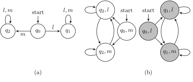
Figure 3: Labelled transition system (a) and behaviour graph (b).

To construct the reduced behaviour graph we carry out deletions of nodes with no successors and for any eventuality clause true⇒

♦

m deletion of nodes where there is no path to a node satisfyingm(see Algorithm 2). To achieve the latter we must find aterminal subgraph Bm, where ¬mholds at each node, from the behaviour graph H. A terminal subgraphBm is one such that

any edge from a node inBm leads to a node also inBm. Thus

♦

m cannot be satisfied on any

path from any node in Bm. So the terminal subgraph must be deleted as it doesn’t satisfy the

eventuality clausetrue⇒

♦

m. In Algorithm 2Delete(Bm), whereBmis a subset of nodes inH,

is a procedure that deletes all the nodes inBmfromH and any edges to, or from, a node inBm.

Algorithm 3 constructs the graph and carries out the deletions.

Theorem 6. Given a TLC(C) formula ϕin Separated Normal Form Algorithm 3 terminates and constructs the reduced behaviour graphHR of ϕ.

Proof. First we show that the outcome of Algorithm 3 is the reduced behaviour graph for ϕ. LetG,H andHR be as in Definition 3 and letH0 be the outcome of Algorithm 1 andHR0 be the

outcome of Algorithm 3, respectively. It should be clear thatH0 is a subgraph of H.

Conversely, consider I1, . . . , In, a path in G such that I1 is an initial node. It can be seen

that I1 ∈Assignments(ψ,C), whereψ=V{Rj |start ⇒Rj is an initial clause inϕ} andIi+1 ∈

Assignments(χi,C), where 16i < nandχi=V{Rk|Lk⇒ gRk is a step clause inϕs.t. Ii|=P L

Lk}. Therefore, by lines 10 and 12 of Algorithm 1, everyIiis a node inH0 andI1, . . . , In is a path

inH0. ThusH is a subgraph ofH0. It can also be seen that if Algorithm 3 deletes a nodeIfrom H0, thenI /∈HR. Finally, it can be seen that if no node can be deleted fromHR0 by Algorithm 3

H_R0 is a reduced behaviour graph.

Next we show that Algorithms 1–3 terminate. Algorithm 1 constructs the behaviour graph. This uses a finite set of clauses and constraints over a finite set of propositions (Props). Nodes are interpretations of Propsthat satisfy the constraints so there are a finite number. In Algorithm 1 the nodes and edges are constructed incrementally. Nodes are marked once they are selected for expansion (line 6) so will not be selected again. Additionally when successors are constructed (lines 7-12) new nodes are only constructed if they do not already exist in the graph. Together this ensures that the algorithm will terminate. Algorithm 2 takes a (finite) subset of nodes of the behaviour graph and deletes those with the required property until there is no change. Hence Algorithm 2 terminates. Algorithm 3 calls Algorithm 1 which terminates and repeatedly carries out deletions until the graph does not change. Again, as the graph is finite this must terminate.

4.3. Example

We illustrate the concept of a behaviour graph and the working of the algorithms by modelling a labelled transition system. Consider the transition system given in Fig. 3(a). Its evolution can be characterised by the following TLC(C) formula in Separated Normal Form

start⇒q0 (q0∧l) ⇒ gq1 (q1∧l) ⇒ gq1 (q2∧l) ⇒ gq2

where the set of constraints is

C={{q0, q1, q2}=1,{l, m}=1}.

(That is, at every moment the system is in exactly one state performing exactly one transition.) In addition, we require that the stateq1 is visited infinitely often.

true⇒

♦

q1

Now, forψ=q0 (notice thatstart ⇒q0is the only initial clause),

Assignments(q0,C) ={{q0, l},{q0, m}}. Thus, the behaviour graph forφcontains two initial nodes, {q0, l}, {q0, m}, both of which are initially unmarked. Suppose{q0, l} is chosen first in line 6 of

Algorithm 1. Then χ = q1 and Assignments(q1,C) = {{q1, l},{q1, m}}, which are added to the

graph. Similarly,{{q2, l},{q2, m}}are introduced as successors of{q0, m}. The algorithm proceeds

and constructs the behaviour graph depicted in Fig. 3(b). It is not hard to see that the reduced behaviour graph obtained in Algorithm 3 by eliminating nodes not satisfying the eventuality only contains nodes{q0, l},{q1, l} and{q1, m} shaded grey in Fig. 3(b), i.e. the formula and the

constraints are satisfiable.

5. BeTL: a Satisfiability Checker for TLC

BeTL (Behaviour graph for Temporal Logic) is a prototype satisfiability checker we have de-veloped that implements the incremental behaviour graph construction algorithm given in Algo-rithm 3 of Section 4. As input it accepts a TLC formula and a set of constraints. BeTL is written in JavaTM programming language using JDK (J2SE Development Kit) 5.0.

5.1. Core Algorithm

BeTL implements the algorithms presented in Section 4. The functionAssignments(ψ,C), where ψis a formula in conjunctive normal form (CNF) andCa set of constraints, is implemented using the Davis-Putnam-Logemann-Loveland (DPLL) algorithm [14] to assign the truth values of each proposition in the nodes. Here we require all the truth assignments of the propositions satisfying bothψandC so we need to modify DPLL to return these assignments rather than just the truth or falsity ofψandC. The sets of assignments that satisfy a constraintC is enumerated and then merged with the set of assignments satisfying the already calculated constraints. Each assignment is used to apply the usual unit propagation toψ.

Algorithm 4 gives the function call DPmod(Γ,Σ) which implements Assignments(ψ,C). This

function takes Γ, a set of sets of literals which satisfy the constraints C, and Σ, a set of sets of literals representing the CNF formulaψ. For example, to compute

Assignments((¬a∨b)∧(¬b∨ ¬c),{{a, b, c}=1_})

we would call call DPmod(Γ,Σ) where

Γ ={{a,¬b,¬c},{¬a, b,¬c},{¬a,¬b, c}} and Σ ={{¬a, b},{¬b,¬c}}.

For each set of the literals that satisfy the constraints (α), the usual unit propagation algorithm, UP(l,Σ) in Algorithm 5 is called for eachl∈α. This deletes sets of literals from Σ that contain l and deletes¬l from any other sets. ∆ is used to store the sets of assignments that satisfy both the sets of constraints and the CNF formula represented by Σ.

In Algorithm 6 the DPmodalgorithm is given which is almost identical to the original DPLL

algorithm [14]. The difference is that, instead of returning ‘satisfiable’ or ‘unsatisfiable’, DPmod

Algorithm 4call DPmod(Γ,Σ) 1: Let ∆ ={}

2: foreachα∈Γdo 3: Σα= Σ

4: foreach literall∈αdo 5: Σα:= UP(l,Σα) 6: end for

7: ∆ = ∆∪DPmod(α,Σα) 8: end for

9: return∆

Algorithm 5UP(l,Σ)

1: foreachα∈Σdo

2: if α={}then return {{}} 3: if l∈αthenΣ := Σ−α

4: if ¬l∈αthenα=α− {¬l} 5: end for

6: returnΣ

5.2. Example

Continuing the example in Section 4.3. Recall that

C={{q0, q1, q2}=1,{l, m}=1}.

The literals satisfying the constraints are enumerated as follows.

Γ = {{q0,¬q1,¬q2, l,¬m},{q0,¬q1,¬q2,¬l, m},{¬q0, q1,¬q2, l,¬m},{¬q0, q1,¬q2,¬l, m}, {¬q0,¬q1, q2, l,¬m},{¬q0,¬q1, q2,¬l, m}}

To construct the initial nodes we must evaluateAssignments(q0,C) and do this by callingcall DPmod(Γ,{{q0}}).

In step 1 of the Algorithm 4 we set ∆ ={}. Then in step 2 letα={q0,¬q1,¬q2, l,¬m}, and in

step 3 set Σα={{q0}}. Steps 4, 5, 6, unit propagateq0, ¬q1,¬q2, l and¬mthrough Σα in turn

as follows.

Σα = U P(q0,Σα) ={}

Σα = U P(¬q1,{}) =U P(¬q2,{}) =U P(¬m,{}) =U P(l,{}) ={}

On line 7 of Algorithm 4

DPmod({q0,¬q1,¬q2, l,¬m},{}) ={{q0,¬q1,¬q2, l,¬m}}

so

∆ ={{q0,¬q1,¬q2, l,¬m}}.

Next time round the loop where

α={q0,¬q1,¬q2,¬l, m}

similarly on line 7 we obtain

DPmod({q0,¬q1,¬q2,¬l, m},{}) ={{q0,¬q1,¬q2,¬l, m}}

Algorithm 6DPmod(β,Σ)

1: (Sat)if Σ ={}then return{β} 2: (Empty)if {} ∈Σthen return{}

3: (Unit propagation)if {l} ∈Σthen return DPmod(β∪ {l},UP(l,Σ)) 4: (Split)if α∈Σand l∈αthen

so

∆ ={{q0,¬q1,¬q2, l,¬m},{q0,¬q1,¬q2,¬l, m}}.

Next when

α={¬q0, q1,¬q2, l,¬m}

on line 6

Σα=U P(¬q0,{{q0}}) ={{}}

and at the end of the for loop on line 6

Σα={{}}.

Now on line 7

DPmod({¬q0, q1,¬q2,¬l, m},{{}}={}

so

∆ = {{q0,¬q1,¬q2, l,¬m},{q0,¬q1,¬q2,¬l, m}} ∪ {}

= {{q0,¬q1,¬q2, l,¬m},{q0,¬q1,¬q2,¬l, m}}.

The remaining values forαare similar and at the end of line 6, Σα={{}}in each case. In line 7

DPmod(α,{{}}={}and so

∆ ={{q0,¬q1,¬q2, l,¬m},{q0,¬q1,¬q2,¬l, m}}

is returned. This is the same as the result returned fromAssignments(q0,C) in Section 4.3. Similar

steps are carried out each timeAssignments(χ,C) is called for different values ofχ.

5.3. Experiments

We have successfully applied BeTL to the temporal specifications stemming from case studies considered in Section 31. In all cases it took BeTL under 600 seconds to compute the expected answer on a PC with a 2.13 GHz Intel Core 2 Duo E6400 processor, 3GB main memory, and 5GB virtual memory running Fedora release 9 with a 32-bit Linux kernel. However, it is important to re-affirm that BeTL is essentially aprototype. It is intended to be the first implementation of a TLC satisfiability checker, and to provide a benchmark for subsequent, more efficient, systems.

In order to evaluate BeTL’s performance, we compared it with two existing PTL tableau the-orem provers, the Logics Workbench (LWB) [39] and the Tableau Work Bench (TWB) [1], on a number of randomly generated benchmark problems. The Logics Workbench [39] is a suite of logi-cal tools for propositional modal and temporal logics including PTL. Here we use thesatisfiability

function in the PTL module that implements Janssen’s tableau algorithm [40] which constructs a tableau using a two pass style algorithm, first constructing the tableau and then deleting nodes. The implementation of Janssen’s algorithm from the LWB is selected over that of Schwendimann’s One Pass Tableau [51] (the LWBmodel function) as our implementation is also a two pass style. The Tableau Workbench [1] is a framework for constructing tableau provers for arbitrary proposi-tional logics. It has a several modules with pre-defined calculi for a number of modal and temporal logics including PTL. We selected these implementations as they are both tableau-based, stable and easily available. We have focussed on tableau-based implementations rather than other styles of prover, eg resolution, so as to focus on the effect of the constraints rather than the algorithms or engineering of particular implementations. Other implementations of PTL provers are discussed further in Section 6.1. We translate the constraints into PTL formulae using the direct encoding as described in Section 2.4.

All of the experiments have been performed on the above mentioned PC. The time was limited to 600 seconds so a time in the table of>600 indicates it did not finish within the allocated time. Any row in the table labelled constraints with entriesn/mdenotes that the problem containedn constrained propositions andmunconstrained propositions.

1_{Problem files can be found at}

Randomly Generated Formulae. We considered 10 sets of benchmarks, where each set contains 100 randomly generated formulae. All formulae are generated using the following criteria:

• The total number of propositions is 10.

• The total number of initial and step clauses added together is 4 clauses.

• The maximum length of each clause is 5, i.e., there can be at most 5 propositions in a clause and, in the case of step clause, the number of propositions on the right and left hand sides are randomly determined.

• Each proposition generated may be negated with the probability 0.5.

• There is only 1 constrained set.

• There are 10 sometimes clauses; one for each proposition in the specification.

The difference between each set is the number of constrained literals, meaning, in the first set, 1 literal is constrained and 9 unconstrained, where, in the sixth set, say, there are 6 constrained and 4 unconstrained propositions.

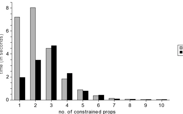
Below is the results of running BeTL, LWB [39] and TWB [1] on the 10 benchmark sets mentioned above. Note that in most cases, TWB did not finish within the 10-minute running time limit. Thus, in such cases, the value of ‘>600’ seconds is used for the purpose of this comparison.

1 2 3 4 5 6 7 8 9 10

BeTL 7.220 8.026 4.487 1.833 0.902 0.387 0.142 0.078 0.055 0.043

LWB 1.960 3.482 4.732 2.319 0.792 0.432 0.097 0.065 0.048 0.044

[image:19.612.115.488.318.370.2]

TWB 102.037 194.001 >600 >600 198.012 198.005 196.001 195.185 >600 196.034

Table 1: Average running time (in seconds) of BeTL, LWB and TWB on the benchmark sets

Figure 4: Comparison graph between BeTL and LWB on the benchmark sets

The experimental results in Table 1 show that the performance of BeTL gradually improves as the number of constrained literals in the specification increases. Since the timings for TWB are greater than for either BeTL or LWB, it is excluded in the comparison graph (Figure 4).

Random State Machines. In Table 2, we show BeTL’s performance on specifications representing randomly generated state transition systems with 5, 10, 15 and 20 states. For example, if a staten1

in the transition system had edges to statesn2andn3this would be represented by the temporal

[image:19.612.95.396.428.617.2]

transition system. There is one constraint {pn1, pn2, . . . pnk}

=1 _{wherek represents the number of}

states in the transition system. Additionally we include formulae that specify that all the states in the system are visited infinitely often. Note that TWB is not included, because its overall results are very slow.

5 states 10 states 15 states 20 states

BeTL 0.017 0.053 0.104 0.375

[image:20.612.192.413.123.160.2]

LWB 0.054 0.131 0.130 14.694

Table 2: Average running time (in seconds) of BeTL, LWB for the transition systems

Overlapping Constraints. We next consider three randomly generated sets of formulae where some literals occur in more than one constraint. We provide three parameters for each experiment of the form (sum, coverage, overlap) where if the three sets areC1,C2,C3

sum = |C1|+|C2|+|C3|

coverage = |(C1∪C2∪C3)|

overlap = |(C1∩C2)|+|(C1∩C3)|+|(C2∩C3))|

One set of formulae is considered in each of Tables 3-5 with differing sets of constraints in each column (a), (b) and (c).

Set1 contains 10 propositions, 10 initial clauses, 20 step clauses, 4 eventualities, maximum clause length is 5. Each set has three constraintsC=1

1 , C2=1,C3=1. All sets are satisfiable.

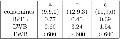
Set2 contains 10 propositions, 10 initial clauses, 20 step clauses, 4 eventualities, maximum clause length is 5. Each set has three constraintsC=2

1 , C2=2,C3=2. All sets are satisfiable.

Set3 contains 15 propositions, 10 initial clauses, 20 step clauses, 5 eventualities, maximum clause length is 5. Each set has three constraintsC1=1, C2=1,C3=1. All sets are satisfiable.

a b c

constraints (6,6,0) (9,6,3) (12,6,6)

BeTL 0.91 0.43 0.44

LWB 35.67 7.24 2.61

[image:20.612.209.395.423.488.2]

TWB >600 >600 >600

Table 3: Running time (in seconds) of BeTL, LWB and TWB on overlapping constraints Set1

a b c

constraints (9,9,0) (12,9,3) (15,9,6)

BeTL 0.77 0.40 0.39

LWB 2.60 3.24 1.54

TWB >600 >600 >600

Table 4: Running time (in seconds) of BeTL, LWB and TWB on overlapping constraints Set2

In each case TWB did not finish within the 10-minute running time limit and BeTL outperforms LWB.

[image:20.612.206.399.536.599.2]

a b c constraints (12,12,0) (15,12,3) (18,12,6)

BeTL 4.30 2.12 1.48

LWB 273.37 155.27 59.38

[image:21.612.196.409.63.126.2]

TWB >600 >600 >600

Table 5: Running time (in seconds) of BeTL, LWB and TWB on overlapping constraints Set3

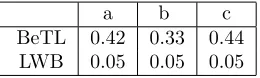
a b c

[image:21.612.238.368.165.204.2]

BeTL 0.42 0.33 0.44 LWB 0.05 0.05 0.05

Table 6: Running time (in seconds) of BeTL and LWB on the Petri Net with Four Philosophers

5.4. Discussion.

We must yet again highlight that BeTL is a prototype and was developed as a first imple-mentation not focusing on any fine tuning of performance. However, we have found that BeTL outperforms TWB on all the problems we considered—we note that that TWB was designed pri-marily for modularity and extensibility rather than efficiency [1]. Further, from Table 1 where the constraints include 8 or more of the 10 propositions BeTL’s performance is comparable to LWB, which is highly optimised, both being less than 0.1 second. Table 1 also shows that BeTL’s per-formance improves as the set of constraints includes a higher proportion of the set of propositions. We note that Table 1 and Figure 4 show the times for both LWB and BeTL increasing until 2-3 constrained propositions and then decreasing. We believe that this is probably due to the phase transition effect that has been studied in the area of SAT [31]. Essentially under-constrained problems are easily found to be satisfiable by provers and over constrained problems are easily found to be unsatisfiable. Here, adding more constraints makes the sets of formulae more likely to be unsatisfiable and hence easier for both provers to solve. We believe that the time to solve the problems goes up initially for both provers because the phase transition occurs at around 2-3 constraints.

Table 2 shows that BeTL has good performance results even compared to the LWB for for-mulae derived from the transition system examples. Similarly the results from the overlapping constraints, Tables 3-5 show BeTL having good performance as compared to LWB. We note that BeTL is slower than LWB on the Petri Net examples possibly due to the fact that there are more unconstrained propositions.

Whilst these results show the idea of incorporating constraints is promising, we note some issues with the underlying algorithm. Firstly, formulae are required to be in a particular normal form. This is not an issue for problems that are already or nearly in the normal form (e.g., the state transition examples in Table 2). For problems that require translation into the normal form, this may require introduction of some new propositions (to rename complex subformulae) and, this adds to the set of unconstrained propositions, whereas the results above show, BeTL works best when most propositions are constrained.

Regarding the algorithm, it constructs nodes that satisfy the set of constraints and a set of (classical logic) clauses. This has two problems. First, we have to explicitly enumerate sets of propositions that satisfy the set of constraints. Second, although the algorithm only generates reachable states, we are often forced to construct all the states, e.g., when there are no initial clauses. This immediately results in the worst case complexity. Inherently, the incremental be-haviour graph construction adopts a breadth-first style that requires us to construct, and keep in memory, a large number of nodes, resulting in an unavoidable inefficiency.

6. Concluding Remarks

In this paper we have introduced TLC, a propositional temporal logic that allows the specifier to define constraints on how many literals from some set can be satisfied at any one time. This logic represents a combination of standard propositional linear-time temporal logic with constraints relating to restrictions on the number of literals, for particular subsets of literals, at each moment in time. Work on TLC has uncovered a new, and potentially very sophisticated, approach to temporal specification. Rather than concentrating solely on the behaviour of components, the use of TLC encourages specifiers to partition the literals, and also to consider what constraints need to be put upon these partitioned sets. Thus, this leads us towards the approach of engineering

the sets and constraints first,before even addressing the temporal specification of the component behaviours.

We provide a graph construction algorithm to check satisfiability by enumerating only the reachable nodes that satisfy the required constraints. Experiments show that an implementation of this outperforms an existing temporal logic tableau reasoner, TWB. Additionally if a high proportion of the propositions are constrained it can also outperform LWB. However we have identified some issues with the algorithm in that it explicitly evaluates the constraints; in many cases it is forced to construct all the states and it adopts a breath-first expansion style. Overall, BeTL works as an initial prototype, providing the basis for more efficient future developments.

6.1. Related Work

We are not aware of others who have explicitly studied constraints directly in the logic itself, such as those described in this paper, apart from ourselves in earlier work on constrained and

exactly one extensions of PTL [18, 19, 20]. Firstly we consider other provers for propositional linear time temporal logic. We discuss two main approaches to theorem proving in PTL: tableau and resolution. Both are refutation based i.e. to prove a formula (ϕ) is valid it is negated and if the negation (¬ϕ) is unsatisfiable then the original must be valid.

Tableau algorithms for PTL, for example see [33, 58] generally have a construction phase followed by a deletion phase. During the construction phase tableau rules are applied to formulae occurring at nodes in the structure which expand the structure and (mostly) simplify formulae. The deletion phase removes parts of the structure which could never be used to construct a model, for example where eventualities cannot be satisfied. Tableau algorithms for PTL have been implemented as part of both the Logics Workbench [39] and the Tableau Workbench [1].

The Logics Workbench [39] is a suite of logical tools for several propositional modal and temporal logics including PTL. The PTL module offers a number of functions to manipulate formulae including the satisfiability and model functions. The satisfiability function implements Janssen’s tableau algorithm [40]. This is a two phase style algorithm as described above. The

model function implements Schwendimann’s One Pass Tableau [51] where the construction and deletion phases are combined.

The Tableau Workbench [1] is a framework for constructing tableau provers for arbitrary propositional logics. It allows users to specify their own tableau rules and provers based on these rules. It has several modules with pre-defined calculi for a number of modal and temporal logics including PTL. Implementations of both Wolper’s and Schwendimann’s tableau are also available from the Automated Reasoning Group at the Australian National University2.

We have compared our prototype prover with LWB and TWB as they are tableau procedures and ours is tableau-like in that it constructs a structure and then deletes parts of this. Our construction method is different in that it requires formulae to be in a particular normal form, and in the worst case may have to build all the nodes in the construction which will be exponential in the number of unconstrained propositions.

Resolution approaches for PTL tend to first translate formulae into some normal form, termed temporal clauses, for example the one provided in Section 2. Then resolution rules are applied to formulae in the normal form that add new temporal clauses to the temporal clause set. The process terminates when either false is derived or no new temporal clauses can be derived. The temporal resolution algorithm from [28] has been implemented in the prover TRP++ [38]. The

behaviour graph construction we use here (without the constraints) was proposed in [28] as part of the completeness proof. It was proposed as a way of dealing with constraints in [19]. A new resolution decision procedure based on labelled superposition is described in [54]. Additionally powerful tools for constructing automata from PTL formulae also exist [13, 32].

In recent years there has been an interest in the development and application of model check-ers [12], for example, NuSMV [9], SPIN [37], Java Pathfinder [55] and PRISM [35]. Model checkcheck-ers take a model of the system, usually some form of directed graph, and a formula, often in a tem-poral logic such as PTL or the branching time temtem-poral logic CTL, and check that the formula is satisfied on the model. Whilst, in general, there is no way to explicitly input constraints as we have done here it may be possible to encode some types of constraints using the input language of the model. For example, in NuSMV enumerated types are allowed which correspond withexactly oneof these propositions holding at any moment. For example the constraint

Mi=1 = {playingi,restingi,injuredi }=1

in Section 3.1 could be defined as an enumerated type,mode, for each player

mode: {play, rest, injured};

Other constraints may be encoded using the INVAR (invariant) command. Formulae in the scope of the INVAR command must not contain any temporal operators so this could be achieved using thepos(C, k) andneg(C, k) formulae defined in Section 2.4 for constraints of the formC∝k_{. Note}

that Model Checking and deduction (for example tableau and resolution calculi) aim to solve different problems. Deductive methods require a formula or set of formulae as input which are shown to be satisfiable or unsatisfiable. Model Checking requires a model and formula as input and show whether the model satisfies the formula.

Propositional satisfiability (SAT) [15] is the problem of deciding whether it is possible to assign true or false to the propositions in a formula of propositional logic that makes the formula evaluate to true. The Davis-Putnam-Logemann-Loveland (DPLL) procedure [14] mentioned in Section 5 has been used to implement SAT solvers but other methods have also been applied. SAT has been successfully applied to a number of areas and efficient implementations that can deal with thousands of variables have been developed. In this paper we use the DPLL algorithm when generating nodes in the behaviour graph that satisfy the sets of constraints and the right hand sides of a set of step clauses. We have implemented our own version of DPLL here as we want to return all the satisfying assignments rather than just returning just one of these. Another alternative would be to call a SAT solver which allows this. Efficient representation of cardinality constraints as a Boolean satisfiability problem has been extensively studied in the literature [2, 5, 53]. A relevant problem is theweighted satisfiability problem, where one checks if a Boolean circuitCproduces 1 as output on some input values in which exactlykvalues are 1 and the others are 0, wherek is a fixedparameter [29].

Cardinality type constraints also appear in Constraint Satisfaction Problems(CSP), see for example [50]. The paper [56] considers encodings of propositional logic into CSP. The additional constraints on propositions we use in this paper could be encoded similarly. To generate nodes in the behaviour graph an alternative approach would be to encode this as a CSP problem and call a CSP solver.

Mutually exclusive conditions (stemming e.g. from automata representations) and numbers from a fixed range can often be handled through efficient translation — consider, for example, logarithmic encoding or property-driven partitioning used in model checking [52] and SAT [6].

6.2. Future Work

Efficient Implementation. The BeTL implementation is a prototype. It was not intended to compete with other temporal provers but was developed as a first implementation against which to measure refined versions. For this reason we have not extended our experiments further to compare BeTL to one pass tableau systems such as [51] or resolution based systems such as TRP++ [38]. We are currently working on such improved versions of the basic tableau approach and expect these to be orders of magnitude faster than BeTL.

botha temporal formula and constraints as input. Input formulae would not have to be transformed into a specific normal form and the usual tableau rules would be applied to the temporal formulae. In addition new tableau rules would be provided to deal with inferences between the propositional part at each moment in time and the tableau constraints. The advantages of this are not having to first translate any temporal formula into normal form; that it does not explicitly require us to construct sets of propositions that satisfy the constraints; and it gives us the opportunity to develop depth-first type algorithms (i.e. exploring one tableau branch at a time). See, for example [51].

Resolution for “Exactly One”. One interesting variation on our work here involves restricting the logic to allow only “exactly one” sets (and as usual some unconstrained propositions) [18, 20], i.e. all the constraints are of the formC=1

i . As a further restriction we can insist that the sets

of propositions in each Ci are disjoint. We term the new logic TLX where TLX(C1, . . . , Cn) =

TLC(C₁=1, . . . , C_n=1) with the additional restriction of disjointness.

In [20] we devised a temporal resolution calculus for TLX, and established its completeness and complexity. Specifically, if a set of TLX clauses is unsatisfiable, then a contradiction will be deduced within time polynomial in N1×N2× · · · ×Nn×2A where N1 is the size ofC1, N2 is

the size of C2, etc, while Ais the number of unconstrained propositions. TLX has a number of

potential applications, and its relatively low complexity makes fast analysis feasible. Thus, part of our future work is to implement and evaluate such resolution calculi.

The application to other logics. We have studied constraints applied to a combination of temporal and epistemic logics in [21]. We could use similar techniques as developed here to apply to other temporal logics such as CTL [10].

Acknowledgements

The authors were partially supported by EPSRC grants GR/S63182 (Dixon, Konev), EP/D060451 (Dixon), EP/H043594 (Konev), EP/D052548 (Fisher) and EP/F033567 (Fisher). Nietiadi was supported by an ORS scholarship with additional support from the Department of Computer Science at the University of Liverpool. The authors would like to thank the reviewers for their constructive remarks.

References

[1] P. Abate, R. Gore, The tableaux workbench, in: TABLEAUX 03: Automated Reasoning with Analytic Tableaux and Related Methods, volume 2796 ofLNAI, Springer, 2003, pp. 230–236. [2] O. Bailleux, Y. Boufkhad, Efficient CNF encoding of boolean cardinality constraints, in: Ninth International Conference on Principles and Practice of Constraint Programming (CP), volume 2833 ofLNCS, pp. 108–122.

[3] H. Barringer, Up and down the temporal way, The Computer Journal 30 (1987) 134–148. [4] A. Behdenna, C. Dixon, M. Fisher, Deductive verification of simple foraging robotic

be-haviours, International Journal of Intelligent Computing and Cybernetics 2 (2009) 604–643. [5] B. Benhamou, L. Sais, P. Siegel, Two proof procedures for a cardinality based language in propositional calculus, in: Proceedings Symposium on Theoretical Aspects of Computer Science (STACS), Springer, London, UK, 1994, pp. 71–82.

[6] L. Bordeaux, Y. Hamadi, L. Zhang, Propositional satisfiability and constraint programming: A comparative survey, ACM Computing Surveys 38 (2006).

[7] A. Cheng, J. Esparza, J. Palsberg, Complexity results for 1-safe nets, Theoretical Computer Science 147 (1995) 117–136.