R E S E A R C H A R T I C L E
Open Access
A Simple Approach to Ranking Differentially
Expressed Gene Expression Time Courses through
Gaussian Process Regression
Alfredo A Kalaitzis
*and Neil D Lawrence
*Abstract
Background:The analysis of gene expression from time series underpins many biological studies. Two basic forms of analysis recur for data of this type: removing inactive (quiet) genes from the study and determining which genes are differentially expressed. Often these analysis stages are applied disregarding the fact that the data is drawn from a time series. In this paper we propose a simple model for accounting for the underlying temporal nature of the data based on a Gaussian process.
Results:We review Gaussian process (GP) regression for estimating the continuous trajectories underlying in gene expression time-series. We present a simple approach which can be used to filter quiet genes, or for the case of time series in the form of expression ratios, quantify differential expression. We assess via ROC curves the rankings produced by our regression framework and compare them to a recently proposed hierarchical Bayesian model for the analysis of gene expression time-series (BATS). We compare on both simulated and experimental data showing that the proposed approach considerably outperforms the current state of the art.
Conclusions:Gaussian processes offer an attractive trade-off between efficiency and usability for the analysis of microarray time series. The Gaussian process framework offers a natural way of handling biological replicates and missing values and provides confidence intervals along the estimated curves of gene expression. Therefore, we believe Gaussian processes should be a standard tool in the analysis of gene expression time series.
Background
Gene expression profiles give a snapshot of mRNA con-centration levels as encoded by the genes of an organ-ism under given experimental conditions. Early studies of this data often focused on a single point in time which biologists assumed to be critical along the gene regulation process after the perturbation. However, the staticnature of such experiments severely restricts the inferences that can be made about the underlying dyna-mical system.
With the decreasing cost of gene expression microar-rays time series experiments have become commonplace giving a far broader picture of the gene regulation pro-cess. Such time series are often irregularly sampled and may involve differing numbers of replicates at each time point [1]. The experimental conditions under which
gene expression measurements are taken cannot be per-fectly controlled leading the signals of interest to be cor-rupted by noise, either of biological origin or arising through the measurement process.
Primary analysis of gene expression profiles is often dominated by methods targeted atstaticexperiments, i. e. gene expression measured on a single time-point, that treat time as an additional experimental factor [1-6]. However, were possible, it would seem sensible to con-sider methods that can account for the special nature of time course data. Such methods can take advantage of the particular statistical constraints that are imposed on data that is naturally ordered [7-12].
The analysis of gene expression microarray time-series has been a stepping stone to important problems in sys-tems biology such as the genome-wide identification of direct targets of transcription factors [13,14] and the full reconstruction of gene regulatory networks [15,16]. A more comprehensive review on the motivations and * Correspondence: A.Kalaitzis@sheffield.ac.uk; N.Lawrence@dcs.shef.ac.uk
The Sheffield Institute for Translational Neuroscience, 385A Glossop Road, Sheffield, S10 2HQ, UK
methods of analysis of time-course gene expression data can be found in [17].
Testing for Expression
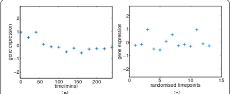
A primary stage of analysis is to characterize the activity of each gene in an experiment. Removing inactive or quiet genes (genes which show negligible changes in mRNA concentration levels in response to treatments/ perturbations) allows the focus to dwell on genes that have responded to treatment. We can consider two experimental set ups. Firstly, we may be attempting to measure the absolute level of gene expression (for exam-ple using Affymetrix GeneChip microarrays). In this case a quiet gene would be one whose expression level is indistinguishable from noise. Alternatively, we might be may be hybridizing two samples to the same array and quantifying the ratio of the expression levels. Here a quiet gene would be one which is showing a similar response in both hybridized samples. In either case we consider such expression profiles will consist principally of noise. Removing such genes will often have benign effects later in the processing pipeline. However, mista-ken removal of profiles can clearly compromise any further downstream analysis. If the temporal nature of the data is ignored, our ability to detect such phenom-ena can be severely compromised. An example can be seen in Figure 1, where the temporal information is removed from an experimental profile by randomly reordering its expression samples. Disregarding the tem-poral correlation between measurements, hinders our ability to assess the profile due to critical inherent traits of the signal being lost such as the speed and scale of variation.
Failure to capture the signal in a profile, irrespective of the amount of embedded noise, may be partially due to temporal aggregationeffects, meaning that the coarse sampling of gene expression or the sampling rates do not match the natural rates of change in mRNA
concentrations [18]. For these reasons, the classification scheme of differential expression in this paper is focused on reaching a hightrue positive rate(TPR, sensitivityor recall ) and is to serve as a pre-processing tool prior to more involved analysis of time-course microarray data. In this work we distinguish between two-sampletesting and experiments where control and treated cases are directly-hybridized on the microarray (For brevity, we shall refer to experiments with such setups as one-sam-ple testing). Thetwo-sample setup is a common experi-mental setup in which two groups of sample replicates are used [13,19]; one being under the treatment effect of interest and the other being the control group, so to recover the most active genes under a treatment one may be interested in testing for the statistical signifi-cance of a treated profile being differentially expressed with respect to its control counterpart. Other studies use data from a one-sample setup [11,12], in which the controland treated cases are directly hybridized on a microarray and the measurements are normalized log fold-changes between the two output channels of the microarray [20], so the analogous goal is to test for the statistical significance of having a non-zero signal.
A recent significant contribution in regards to the esti-mation and ranking of differential expression of time-series in a one-samplesetup is a hierarchical Bayesian model for the analysis of gene expression time-series (BATS) [11,12] which offers fast computations through exact equations of Bayesian inference, but makes a con-siderable number of prior biological assumptions to accomplish this (cf.Simulated data).
Gene Expression Analysis with Gaussian Processes Gaussian processes(GP) [21,22] offer an easy to imple-ment approach to quantifying the true signal and noise embedded in a gene expression time-series, and thus allow us to rank the differential expression of the gene profile. A Gaussian process is the natural generalisation of a multivariate Gaussian distribution to a Gaussian distribution overa specific family of functions–a family defined by acovariance functionor kernel, i.e. a metric of similarity between data-points (Roughly speaking, if we also view a function as a vector with an infinite number of components, then that function can be repre-sented as a point in an infinite-dimensionalspace of a specific family of functionsand a Gaussian process as an infinite-dimensional Gaussian distribution over that space).
In the context of expression trajectory estimation, a Gaussian process coupled with the squared-exponential covariance function (orradial basis function, RBF) –a standard covariance function used in regression tasks– makes the reasonable assumption that the underlying true signal in a profile is a smoothfunction [23], i.e. a
0 50 100 150 200 −2
−1 0 1 2
time(mins)
gene expression
0 5 10 15
−2 −1 0 1 2
randomised timepoints
gene expression
[image:2.595.56.292.563.660.2]
function with an infinite degree of differentiability. This property endows the GP with a large degree of flexibility in capturing the underlying signals without imposing strong modeling assumptions (e.g. number of basis func-tions) but may also erroneously pick up spurious pat-terns (false positives) should the time-course profiles suffer from temporal aggregation. From a generative viewpoint, the profiles are assumed to have been cor-rupted by additive white Gaussian noise. This property makes the GP an attractive tool for bootstrapping simu-lated biological replicates [24].
In a different context, Gaussian process priors have been used for modeling transcriptional regulation. For example in [25], while using the time-course expression of a-priori known direct targets (genes) of a transcrip-tion-factor, the authors went one step further and inferred the concentration rates of the transcription-fac-tor protein itself and [26] extended the same model for the case of regulatory repression. The ever-lingering issue of outliers in time series is still critical, but is not addressed here as there is significant literature on this issue in the context of GP regression, which is comple-mentary to this work.
For example [19,27] developed a probabilistic model using Gaussian processes with a robust noise model spe-cialised for two-sample testing to detectintervalsof dif-ferential expression, whereas the present work optionally focuses on one-sampletesting, to rank the differential expression and ultimately detectquiet/active genes. Other examples can also be easily applied; [28] use a Student-tdistribution as the robust noise model in the regression framework along with variational approximations to make inference tractable, and [29] employ a Student-t observation model with Laplace approximations for inference. The standard GP regres-sion framework is straightforward to use here with a limited need for manual tweaking of a few hyper-para-meters. We describe the GP framework, as used here for regression, in more detail in theMethodssection.
Results and Discussion
We apply standard Gaussian process (GP) regression and the Bayesian hierarchical model for the analysis of time-series (BATS) on two in-silico datasets simulated by BATS and GPs, and on one experimental dataset coming from a study on primary mouse keratinocytes with an induced activation of the TRP63 transcription factor, for which a reverse-engineering algorithm was developed (TSNI: time-series network identification) to infer the direct targets of TRP63 [13].
We assume that each gene expression profile can be categorized as either quiet or differentially expressed. We consider algorithms that provide a rank ordering of the profiles according to which is most likely to be
non-quiet (or differentially expressed). Given ground truth we can then evaluate the quality of such a ranking and compare different algorithms. We make use ofreceiver operating characteristic curves (ROC curves) to evaluate the algorithms. These curves plot the false positive rate on the horizontal axis, versus the true positive rateon the vertical axis; i.e. the percentage of the total negatives (non-differentially expressed profiles) erroneously classi-fied as positives (differentially expressed) versus the per-centage of the total positives correctly classified as positives.
From the output of each model a ranking of differen-tial expression is produced and assessed with ROC curves to quantify how well in accordance to each of the three ground truths (BATS-sampled, GP-sampled, TSNI-experimental) the method performs. The BATS model can employ three different noise models, where the marginal distribution of the error is assumed to be either Gaussian, Student-tor double exponential respec-tively. For the following comparisons we plot four ROC curves, one for each noise model of BATS and one for the GP. We demonstrate that the ranking of the GP fra-mework outperforms that of BATS with respect to the TSNI ranking on the experimental data and on GP-sampled profiles.
Simulated data
The first set of in-silico profiles are simulated by the BATS software http://www.na.iac.cnr.it/bats/ in accor-dance to the guidelines given in [12]. In BATS [11] each time-course profile is assumed to be generated by a function expanded in an orthonormal basis (Legendre or Fourier) plus noise. The number of bases and their coef-ficients, are estimated with analytic computations in a fully Bayesian manner. Thus the global estimand for every gene expression trajectory is the linear combina-tion of some number of bases whose coefficients are estimated by a posterior distribution. In addition, the BATS framework allows various types of non-Gaussian noise models.
BATS simulation
We reproduce one instantiation of the simulations per-formed in [11]; specifically, three sets ofN= 8000 pro-files, of n= 11 timepoints and kji= 2replicates, for i= 1; ..., N, j = 1, ..., nexcept k2,5,7i = 3,according to the model defined in [11, sec. 2.2]. In each of the three sets of profiles, 600 out of 8000 are randomly chosen to be differentially expressed (labeled as “1” in the ground truth) and simulated as a sum of an orthonormal basis of Legendre polynomials with additive i.i.d.(identically and independently distributed) noise.
functions with additive i.i.d. noise. The three simulated datasets are induced with different kinds of i.i.d. noise; respectively, Gaussian N(0, s2), Student-tdistributed with 5(T(5)) and 3 (T(3)) degrees of freedom. Figure 2 (a, b, c) illustrates the comparison on the BATS-sampled data with all three kinds of induced noise.
GP simulation
In a similar setup, the second in-silico dataset consists of 8000 profiles sampled from Gaussian processes, with the same number of replicates and time-points, among which 600 were setup as differentially expressed. To generate a differentially expressed profile, each of the hyperparametersof the RBF covariance function, namely thecharacteristic lengthscale, signal variance andnoise
variance (cf. Methods) is sampled from separate Gamma distributions. The three Gamma distributions are fitted to sets of their corresponding hyperpara-meters, which are observed for the true positive profiles under a near zero FPR during the first test on BATS-generated profiles. In this way, we attempt to resemble the behaviour of the BATS-sampled profiles. Table 1 lists the parameters of the three fitted Gamma distributions.
The other 7400 non-differentially expressed profiles are simply zero functions with additive white Gaussian noise of variance equal to the sum of two samples from the Gamma distribution for thesignal varianceand the noise variance. This addition serves to create a
non-0
0.2
0.4
0.6
0.8
1
0
0.2
0.4
0.6
0.8
1
FPR
TPR
GP (auc=0.922)
BATS
G(auc=0.984)
BATS
T(auc=0.981)
BATS
DE(auc=0.981)
0
0.2
0.4
0.6
0.8
1
0
0.2
0.4
0.6
0.8
1
FPR
TPR
GP (auc=0.931)
BATS
G(auc=0.977)
BATS
T(auc=0.982)
BATS
DE(auc=0.980)
0
0.2
0.4
0.6
0.8
1
0
0.2
0.4
0.6
0.8
1
FPR
TPR
GP (auc=0.937)
BATS
G(auc=0.973)
BATS
T(auc=0.976)
BATS
DE(auc=0.973)
0
0.2
0.4
0.6
0.8
1
0
0.2
0.4
0.6
0.8
1
FPR
TPR
GP (auc=0.944)
BATS
G(auc=0.749)
BATS
T(auc=0.825)
BATS
DE(auc=0.816)
[image:4.595.60.540.90.491.2]differentiated profile of comparative scale to the differ-entiated ones, but nonetheless of completely random nature. Figure 2(d) illustrates the comparison on the GP-sampled data.
Experimental data
We apply the standard GP regression framework and BATS on an experimental dataset coming from a study on primary mouse keratinocytes with an induced activa-tion of the TRP63 transcripactiva-tion factor (GEO-accession number [GEOdataset:GSE10562]), where a reverse-engi-neering algorithm was developed (TSNI: time-series net-work identification) to infer the direct targets of TRP63 [13]. In that study, 786 out of 22690 gene reporters were chosen based on the area under their curves, and ranked by TSNI according to the probability of belong-ing to direct targets of TRP63. The rankbelong-ing list was pub-lished in a supplementary file available for download
(genome.cshlp.org/content/suppl/2008/05/05/ gr.073601.107.DC1/DellaGatta_SupTable1.xls) and used here as anoisy ground truth. We pre-process the data with the robust multi-array average (RMA) expression measure [30], implemented in the“affy”R-package.
We label the top 100 position of the TSNI ranking as
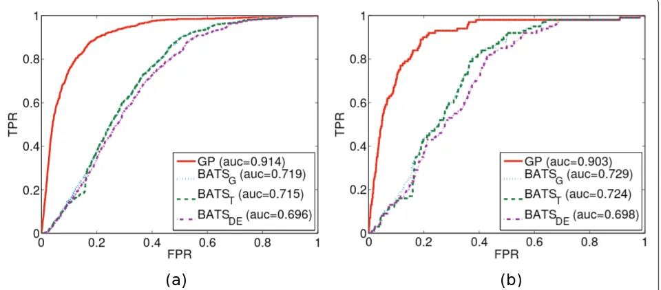
[image:5.595.57.539.101.185.2]“1”in the ground truth as they are the most likely to be direct targets of the TRP63 transcription factor and because the binding scores (computed as the sum of -log2 ofp-values of all TRP63-binding regions identified by ChIP-chip experiments) are most densely distributed amongst the first 100 positions, see Figure 3. Further-more, in [13] these 100 positions were further validated by gene set enrichment analysis (GSEA) [31] to check if their up/down regulation patterns were correlated to genes that respond to TRP63 knock-downs in general. In summary,“the top 100 TSNI ranked transcripts are significantly enriched for the strongest binding sites”[13]. Figure 4 illustrates the comparison on the experimental data.
Discussion
On BATS-sampled data, Figure 2(a, b, c), we observe that the change in the induced noise is barely noticeable
in regards to the performances of both methods and that BATS maintains its stable supremacy over the GP framework. This performance gap is partially due to the lack of a robust noise model for the GP (cf. Conclu-sions). Furthermore, there is a modeling bias in the underlying functions of the simulated profiles, which contain a finite small degree of differentiability (maxi-mum degree of Legendre polynomial is 6). This puts the GP in a disadvantaged position as it models for (smooth) infinitely differentiable functions when its cov-ariance function is a squared exponential. Consequently, for this simulated dataset the GP is more susceptible to capturing spurious patterns as they are more likely to lie within its modeling range, whereas for BATS modeling the polynomials with a limited degree acts as a safe-guard against spurious patterns, most of which vary rapidly in time.
On GP-sampled data, Figure 2(d), we observe the reversal of the performance gap in favor of the GP fra-mework while its performance is almost unaffected. The Table 1 Parameters of the Gamma distributions for sampling the RBF-hyperparameters
Sampling Gamma distributionΓ(a,b)
a(scale) b(shape)
Sampled
RBF-Hyperparameters
ℓ2(characteristic lengthscale) 1.4 5.7
σ2
f(signal variance) 2.76 0.2
σ2
n(noise variance) 23 0.008
These are the parameters of the Gamma distributions from which we sample the RBF- hyperparameters. For example, the characteristic lengthscale is sampled from a Gamma with scale 1.4 and shape 5.7. The hyperparameters are then used in the RBF covariance function to sample/simulate a profile from the Gaussian process.
[image:5.595.305.539.486.664.2]GP is still prone to non-differentially expressed profiles with spurious patterns and differentially expressed pro-files with excessive noise. However, the limited polyno-mial degree of BATS proves to be inadequate for many of the GP-sampled functions and the two BATS variants with robust noise models (BATST, BATSDE) only allevi-ate the problem slightly. In Figure 4 we observe the GP outperforming the Gaussian noise variant of BATS (BATSG) by a similar degree as in Figure 2(d). The experimental data are much more complex and appar-ently the robust BATS variants now offer no increase in performance. Since the ground truth focuses on the 100 most differentially expressed genes with respect to the induction of the TRP63 transcription factor, then these results indicate that the GP method of ranking pre-sented here indeed highlights differentially expressed genes and that it naturally features an attractive degree of robustness against different kinds of noise.
Conclusions
We presented an approach to estimating the continuous trajectory of gene expression time-series from microar-ray data throughGaussian process (GP) regression and ranking the differential expression of each profile via a log-ratio of marginal likelihoods of two GPs, each one representing the hypothesis of differential and non-dif-ferential expression respectively. We compared our method to a recent Bayesian hierarchical model (BATS) via ROC curves on data simulated by BATS and GPs and experimental data. Each evaluation was made on
the basis of matched percentages to a ground truth - a binary vector which labeled the profiles in a dataset as differentially expressed or not. The experimental data were taken from a previous study on primary mouse keratinocytes and the top 100 genes of its ranking were used here as the noisy ground truth for the purposes of assessment. The GP framework significantly outper-formed BATS on experimental and GP-sampled data and the results showed that standard GP regression can be regarded as a serious competitor in evaluating the continuous trajectories of gene expression and ranking its differential expression.
This ranking scheme presented here is reminiscent of the work in [19] on two-sample data (separate time-course profiles for each treatment), where the two com-peting hypotheses are represented in a graphical model of two different generative models connected with a gat-ing scheme; one where the two profiles of the gene reporter are assumed to be generated by two different GPs, and thus the gene isdifferentially expressed across the two treatments, and one where the two profiles are assumed to be generated by the same GP, and thus the gene isnon-differentially expressed. The gating network serves toswitchbetween the two generative models, in time, to detect intervalsof differential expression and thus allow biologists to draw conclusions about the pro-pagation of a perturbation in a gene regulatory network. Instead, the issue presented in this paper is more basic and so is the methodology to deal with it. However, we note that the robust mechanisms against outliers used
0 0.2 0.4 0.6 0.8 1
0 0.2 0.4 0.6 0.8 1
FPR
TPR
GP (auc=0.914) BATSG(auc=0.719) BATST(auc=0.715) BATSDE(auc=0.696)
0 0.2 0.4 0.6 0.8 1
0 0.2 0.4 0.6 0.8 1
FPR
TPR
GP (auc=0.903) BATSG(auc=0.729) BATST(auc=0.724) BATSDE(auc=0.698)
[image:6.595.60.540.463.674.2]in [19,28,29] are complementary to this work and one should not hesitate to incorporate one into a framework similar to ours. Practicalities aside, this paper also intro-duces additional proof that Gaussian processes, naturally and without much engineering, fit to the analysis of gene expression time-series and that simplicity can still be preferred over the ever-increasing –but sometimes
necessary – complexity of hierarchical Bayesian
frameworks.
Future work
A natural next step would be to add a robust noise mechanism in our framework. In this regard, fine exam-ples can be found in [19,28,29]. Finally, an interesting biological question is about the potential periodicity of the underlying signal in a gene expression profile. In this regard a different of kind stationary covariance function, theperiodiccovariance function [22], can fit a time-series generated by an periodic process and thus its lengthscale hyperparameter can be interpreted as its cycle.
Methods
As we mentioned earlier, analysing time-course microar-ray data by means of Gaussian process (GP) regression is not a new idea (cf.Background). In this section we review the methodology to estimating the continuous trajectory of a gene expression by GP regression and subsequently describe a likelihood-ratio approach to ranking the differential expression of its profile. The fol-lowing content is based on the key components of GP theory as described in [21,22].
The Gaussian process model
The idea is to treat trajectory estimation given the observations (gene expression time-series) as an interpo-lation problem on functions of one dimension. By assuming the observations have Gaussian-distributed noise, the computations for prediction become tractable and involve only the manipulation of linear algebra rules.
A finite parametric model
We begin the derivation of the GP regression model by defining a standardlinear regressionmodel (a more con-crete example of such a model is forj= (1, x,x2)⊤, i.e. a line mapped to a quadratic curve)
f(x) =φTw, y=f(x) +ε, (1)
where gene expression measurements in timey= {yn}n
= 1..N are contaminated with white Gaussian noise and the inputs (of time) are mapped to a feature space F= {j(xn)⊤}n= 1..N. Furthermore, if we assume the noise to be i.i.d. (identically and independently distributed) as a
Gaussian with zero mean and varianceσn2
∼N(0,σ2
n), (2)
then the probability density of the observations given the inputs and parameters (data likelihood) is Gaussian-distributed
p(y|x,w) = n
i=1
p(yi|xi,w)
= n
i=1 1
2πσ2 n
exp
−(yi−φiw)
2
2σ2 n
= 1
(2π)n/2|n|1/2×
exp
−1
2(y−w)
−1(y−w)
=N(w,n),
(3)
Wheren=σn2I.
Introducing Bayesian methodology
Now turning to Bayesian linear regression, we wish to encode our initial beliefs about the parameters wby specifying a zero mean, isotropic Gaussian distribution as apriorover the parameters
w∼N(0,σ2
w). (4)
By integrating the product of the likelihood × prior with respect to the parameters, we get themarginal like-lihood
p(y|x) =
dwp(y|x,w)p(w), (5)
which is jointly Gaussian. Hence themeanand covar-ianceof themarginalare
y=w+ε=0 (6)
yy=ww+εε
=σw2+σn2I
=Kf +σn2I=Ky
(7)
p(y|x) = 1 (2π)n/2|Ky|1/2
exp
−1
2y
K−1 y y
=N(y;0,Ky).
(8)
Notice in eq. (7) how the structure of the covariance implies that choosing a different feature spaceFresults in a differentKy. Whatever Kyis, it must satisfy the fol-lowing requirements to be a valid covariance matrix of the GP:
• Kolmogorov consistency, which is satisfied when Kij =K(xi,xj) for somecovariance function K, such that all possibleKarepositive semidefinite (y⊤Ky≥ 0).
• Exchangeability, which is satisfied when the data are i.i.d.. It means that the order in which the data become available has no impact on themarginal dis-tribution, hence there is no need to hold out data from the training set for validation purposes (for measuring generalisation errors, etc.).
Definition of a Gaussian process
More formally,a Gaussian process is a stochastic process (or collection of random variables) over a feature space, such that the distribution p (y(x1), y(x2),..., y(xn)) of a function y(x), for any finite set of points{x1, x2, ...,xn} mapped to that space, is Gaussian, and such that any of these Gaussian distributions is Kolmogorov consistent.
If we remove thenoise termσ2
nIfromKyin eq. (7) we can have noiseless predictions off(x) rather thany(x) =f (x) + ε. However, when dealing with finite parameter spacesKfmay beill-conditioned (cf. sec.SE derivation), so thenoise termguarantees that Kywill havefull rank (and an inverse). Having said that, we now formulate the GPpriorover thelatentfunction valuesfby rewrit-ing eq. (8) as
p(f|x) = 1 (2π)n/2|
Kf|1/2×
exp
−1
2(f−m)
K−1 f (f−m)
,
orf|x∼GP (f;m(x), Kf(xi,xj)),
(9)
where themean function(usually defined as the zero function) and thecovariance functionrespectively are
m(x) =f(x), (10)
Kf(xi,xj) =(f(xi)−m(xi))(f(xj)−m(xj)). (11)
The squared-exponential kernel
In this paper we only use the univariate version of the squared-exponential (SE) kernel. But before embarking on its analysis, the reader should be aware of the exist-ing wide variety of kernel families, and potential combi-nations of them. A comprehensive review of the
literature on covariance functions is found in [21, chap. 4].
Derivation and interpretation of the SE kernel
In the GP definition section we mentioned the possibi-lity of an ill-conditionedcovariance matrix. In the case of a finite parametric model (as in eq. (1)),Kfcan have at most as many non-zero eigenvalues as the number of parameters in the model. Hence for any problem of any given size, the matrix is non-invertible. Ensuring Kfis not ill-conditioned, involves adding the diagonal noise term to the covariance. In an infinite-dimensional fea-ture space, one would not have to worry about this issue as the features are integrated out and the covar-iance between datapoints is no longer expressed in terms of the features but by a covariance function. As demonstrated in [22, sec.45.3] and [21, sec.4.2.1], with an example of a one-dimensional dataset, we express the covariance matrixKfin terms of the featuresF
Kij=σw2 h
φh(xi)φh(xj), (12)
then by considering a feature space defined by radial basis functionsand integrating with respect to their cen-tersh, eq. (12) becomes
K(xi,xj) = lim N→∞
σ2 w N
N
h=1
φh(xi)φh(xj)
=S
∞
−∞dhφh(xi)φh(xj)
=S
∞
−∞dhexp
−(xi−h)2
2r2
exp
−(xj−h)2
2r2
=√πr2Sexp
−(xi−xj)
2
4r2
,
(13)
where one ends up with a smooth (infinitely differenti-able) function on an infinite-dimensional space of (radial basis function) features. Taking the constant out front as asignal varianceσf2and squaring the exponential gives
rise to the standard form of the univariate squared-exponential(SE) covariance function. The noisy univari-ateSE kernel–the one used in this paper is
Ky(xi,xj) =σf2exp
−(xi−xj)2
22
+σn2δij. (14)
The SE is a stationarykernel, i.e. it is a function of d=xi- xjwhich makes ittranslation invariant in time.
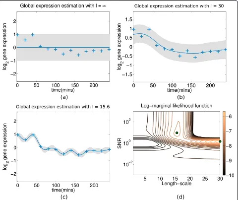
the lengthscalel2governs the amount thatfvaries along the input (time). A small lengthscale means thatfvaries rapidly along time, and a very large lengthscale means that f behaves almost as a constant function, see Figure 5. This parameterisation of the SE kernel becomes very powerful when combined with hyperpara-meter adaptation, as described in a following section.
Other adapted hyperparameters include the signal var-iance σf2which is a vertical scale of function variation and thenoise varianceσ2
n (introduced in eq. (2)) which
is not a hyperparameter of the SE itself, but unless we consider it as a constant in thenoisycase, its adaptation can give different explanations about the latent function that generates the data.
Figure 5 Gaussian process fit on expression profile of gene Cyp1b1 in the experimental mouse data. Figure 5: A GP fitted on the centred profile of the geneCyp1b1(probeID 1416612_at in theGSE10562dataset) with different settings of the lengthscale hyperparameterℓ2.
The blue crosses represent zero-mean hybridised gene expression in time (log2 ratios between treatment and control) and the shaded area indicates the point-wise mean plus/minus two times the standard deviation (95% confidence region).(a)Mean function is constant asℓ2
®∞
(0 inverse lengthscale in eq. (14)) and all of the observed data variance is attributed to noise (σn2).(b)The lengthscale is manually set to a local-optimum large value (ℓ2= 30) and thus the mean function roughly fits the data-points. The observed data variance is equally attributed to
signal (σf2) and noise (σn2). Consequently, the GP features high uncertainty in its predictive curve.(c)The lengthscale is manually set to a local-optimum small value (ℓ2= 15.6) and thus the mean function tighly fits the data-points with high certainty. The interpretation from the
covariance function in this case is that the profile contains a minimal amount of noise and that most of the observed data variance is attributed to the underlying signal (σf2).(d)The contour of the corresponding LML function plotted by an exhaustive search ofℓ2and SNR values. The
One can also combine covariance functions as long as they are positive-definite. Examples of valid combined covariance functions include thesumand convolutionof two covariance functions. In fact, eq. (14) is a combined sum of the SE kernel with the covariance function of isotropic Gaussian noise.
Gaussian process prediction
To interpolate the trajectory of gene expression at non-sampled time-points, as illustrated in Figure 5, we infer a function value f* at a new input (non-sampled time-point)x*, given the knowledge of function estimates fat known time-points x. The joint distribution p(f*, f ) is Gaussian, hence the conditional distributionp(f*| f) is also Gaussian. In this section we consider predictions using noisy observations; we know the noise is Gaussian too, so the noisy conditional distribution does not differ. By Bayes’rule
p(f∗|y) = p(f∗,y)
p(y) , (15)
where the Gaussian process prior over the noisy observations is
p(y) =N(0, cov(y)) =N(0,Kf(x,x) +σn2I) (16)
Predictive equations for GP regression
We start by defining themean functionand the covar-iance between a new time-point x*and each of the ith known time-points, wherei= 1..N
mi=m(xi), (17)
(k∗)i=Kf(xi,x∗). (18)
For every new time-point a new vector k* is concate-nated as an additional row and column to the covar-iance matrixKCto give
KC+1=
[KC] [k∗] [k∗] [κ]
, (19)
where C = N..N* is incremented with every new k* added to KC. By considering a zero mean function and eq. (19), the joint distributionp(f*, y) from eq. (15) can be computed
y f∗
∼N
0,
Kf(X,X) +σ2I Kf(X,X∗)
Kf(X∗,X) Kf(X∗,X∗)
. (20)
Finally, to derive thepredictive mean andcovariance of the posterior distribution from eq. (15) we use the Gaussian identities presented in [21, sec.A.2]. These are
the predictive equations for GP regression of a single new time-point
p(f∗|y)∼N(f∗;m∗,var(f∗)), where (21)
m∗=k∗(Kf+σn2I)−1y, (22)
var(f∗) =k(x∗,x∗)−k∗(Kf+σn2I)−1k∗, (23)
andKf=Kf(x,x). These equations can be generalised easily for the prediction of function values at multiple new time-points by augmenting k*with more columns andk(x*,x*) with more components, one for each new time-pointx*.
Hyperparameter learning
Given the SE covariance function, one can learn the hyperparameters from the data by optimising the log-marginal likelihood function of the GP. In general, a non-parametric model such as the GP can employ a variety of kernel families whose hyperparameters can be adapted with respect to the underlying intensity and fre-quency of the local signal structure, and interpolate it in a probabilistic fashion (i.e. while quantifying the uncer-tainty of prediction). The SE kernel allows one to give intuitive interpretations of the adapted hyperparameters, especially for one-dimensional data such as a gene expression time-series, see Figure 5 for interpretations of various local-optima.
Optimising the marginal likelihood
In the context of GP models the marginal likelihood results from the marginalisation over function valuesf
p(y|x) =
dfp(y|f,x)p(f|x), (24)
where the GP prior p(f|x) is given in eq. (9) and the likelihood is a factorised Gaussian y|f∼N(f,σ2
nI). The
integral can be evaluated analytically [21, sec. A.2] to give the log-marginal likelihood (LML, it is common practice to take the log of the antiderivative for the sake of numerical stability, as it yields a sum instead of a pro-duct)
lnp(y|x,θ) =−1 2y
TK−1 y y−
1
2ln|Ky| − n 2ln 2π, whereKy =Kf +σ2
nI
(25)
∂
∂θ lnp(y|x,θ) = 1 2α
T∂Ky ∂θ α−
1 2tr
K−y1∂Ky ∂θ
= 1 2tr
(αα−K−y1)∂Ky ∂θ
,
whereα = K−y1yand
∂Ky ∂θ =
∂Ky ∂, ∂Ky ∂σ2 f , ∂Ky ∂σ2 n =
Kf(xi−xj) 2
3 , exp
−(xi−xj)2
22
, δij
.
(26)
We use scaled conjugate gradients[32]– a standard optimisation scheme–to maximise the LML.
Ranking with likelihood-ratios
Alternatively, one may choose to go“fully Bayesian”by placing ahyper-prior over the hyperparametersp(θ |H), whereHrepresents some type of model, and compute a posterior over hyperparameters
p(θ|y,x,H) = p(y|x,θ,H)p(θ|H)
∫dθp(y|x,θ,H)p(θ|H), (27)
based on some initial beliefs, such as the functions having large lengthscales, and optimise the marginal likelihood so that the optimum lengthscale tends to a large value, unless there is evidence to the contrary. Depending on the modelH, the integral in eq. (27) may be analytically intractable and thus one has to resort to approximating this quantity [33] (e.g. Laplace
approxi-mation) or using Markov Chain Monte Carlo(MCMC)
methods to sample from the posterior distribution [34]. In the case where one is using different types of mod-els (e.g. with different number of hyperparameters), a Bayesian-standard way of comparing between such two models is through Bayes factors [11,19,23] –ratios of theintegralquantities in eq. (27)
K= ∫dθ1p(y|x,θ1,H1)p(θ1|H1)
∫dθ2p(y|x,θ2,H2)p(θ2|H2)
, (28)
where the modelsHusually represent two different hypotheses, namely H1- the profile has a significant
underlying signal and thus it is truly differentially expressed andH2- there is no underlying signal in the
profile and the observed gene expression is just the effect of random noise. The ranking is based on how likelyH1in comparison toH2, given a profile.
In this paper we present a much simpler–but effec-tive to the task –approach to ranking the differential expression of a profile. Instead of integrating out the hyperparameters, we approximate the Bayes factor with a log-ratio of marginal likelihoods (cf. eq. (25))
ln
p(y|x,θ2) p(y|x,θ1)
, (29)
with each LML being a function of different instantia-tions ofθ. We still maintain hypothesesH1andH2that
represent the same notions explained above, but in our case they differ simply by configurations ofθ. Specifi-cally, on H1the hyperparameters arefixed toθ1 = (∞, 0; var(y))⊤to encode a function constant in time (l2 ®
∞), with no underlying signal(σf2= 0), which generates a time-series with a variance that can be solely explained by noise(σ2
n =var(y)). Analogously, on H2the
hyper-parameters θ2 are initialised to encode a function that fluctuates in accordance to a typical significant profile (e.g.ℓ2 = 20), with a distinct signal variance that solely explains the observed time-series variance(σf2=var(y))
and with no noise(σ2 n = 0).
Local optima of the log-marginal likelihood (LML) function
[image:11.595.68.294.85.229.2]These two configurations correspond to two points in the three-dimensional function that is the LML, both of which usually lie close to local-optimum solutions. This assumption can be verified, empirically, by exhaustively plotting the LML function for a number of profiles, see Figure 5. In case the LML contour differs for some pro-files, more initialisation points should be used to ensure convergence to the maximum-likelihood solution. Because the configuration of the second hypothesis (no noise, σ2
n = 0) is an extremely unlikely scenario, we let θ2adapt to a given profile by optimising the LML func-tion, as opposed to keeping it fixed likeθ1.
In most cases the LML (eq. (25)) is not convex. Multi-ple optima do not necessarily pose a threat here; depending on the data and as long as they have similar function values, multiple optima present alternative interpretations on the observations. To alleviate the pro-blem of spurious local optimum solutions however, we make the following observation: when we explicitly restrict the signal variance hyperparameter (σf2) to low
values during optimisation, we also implicitly restrict the noise variance hyperparameter (σf2) to large values. This occurs as the explanation of the observed data variance (var(y)) is shared between the signal and noise variance hyperparameters, i.e.var(y)σ2
f +σn2. This dependency
allows us to treat the three-dimension optimisation pro-blem as a two-dimension propro-blem, one of lengthscale ℓ
2
and one of signal-to-noise ratioSNR= σ 2 f σ2
n
without fear
of missing out an optima.
with a relatively complex function and a small noise var-iance, and one optimum for a large lengthscale and a low SNR, where the data are explained by a simpler function with high noise variance. We also notice that the first optimum has a lower LML. This relates to the algebraic structure of the LML (eq. (25)); the first term (dot product) promotes data fitness and the second term (determinant) penalizes the complexity of the model [21, sec.5.4]. Overall, the LML function of the Gaussian process offers a good fitness-complexity trade-off without the need for additional regularisation. Optionally, one can use multiple initialisation points focusing on different non-infinite lengthscales to deal with the multiple local optima along the lengthscale axis, and pick the best solution (max LML) to represent the H1hypothesis in the likelihood-ratio during the
ranking stage.
Source code
The source code for the GP regression framework is available in MATLAB code http://staffwww.dcs.shef.ac. uk/people/N.Lawrence/gp/ and as a package for the R statistical computing language http://cran.r-project.org/ web/packages/gptk/. The routines for the estimation and ranking of the gene expression time-series are available upon request for both languages. The time needed to analyse the 22690 profiles in the experimental data, with only the basic two initialisation points of hyperpara-meters, is about 30 minutes on a desktop running Ubuntu 10.04 with a dual-core CPU at 2.8 GHz and 3.2 GiB of memory.
Acknowledgements
The authors would like to thank Diego di Bernardo for his useful feedback on the experimental data. Research was partially supported by a EPSRC Doctoral Training Award, the Department of Neuroscience, University of Sheffield and BBSRC (grant BB/H018123/2).
Authors’contributions
AAK designed and implemented the computational analysis and ranking scheme presented here, assessed the various methods and drafted the manuscript. NDL pre-processed the experimental data and wrote the original Gaussian process toolkit for MATLAB and AAK rewrote it for the R statistical language. Both AAK and NDL participated in interpreting the results and revising the manuscript. All authors read and approved the final manuscript.
Received: 18 January 2011 Accepted: 20 May 2011 Published: 20 May 2011
References
1. Lönnstedt I, Speed TP:Replicated microarray data.Statistica Sinica2002,
12:31-46.
2. Spellman PT, Sherlock G, Zhang MQ, Iyer VR, Anders K, Eisen MB, Brown PO, Botstein D, Futcher B:Comprehensive identification of cell cycle-regulated genes of the yeast Saccharomyces cerevisiae by microarray hybridization.Molecular biology of the cell1998,9(12):3273.
3. Friedman N, Linial M, Nachman I, Pe’er D:Using Bayesian networks to analyze expression data.Journal of computational biology2000, 7(3-4):601-620.
4. Dudoit S, Yang YH, Callow MJ, Speed TP:Statistical methods for identifying differentially expressed genes in replicated cDNA microarray experiments.Statistica sinica2002,12:111-140.
5. Kerr MK, Martin M, Churchill GA:Analysis of variance for gene expression microarray data.Journal of Computational Biology2000,7(6):819-837. 6. Efron B, Tibshirani R, Storey JD, Tusher V:Empirical Bayes analysis of a
microarray experiment.Journal of the American Statistical Association2001,
96(456):1151-1160.
7. Bar-Joseph Z, Gerber G, Simon I, Gifford DK, Jaakkola TS:Comparing the continuous representation of time-series expression profiles to identify differentially expressed genes.Proceedings of the National Academy of Sciences of the United States of America2003,100(18):10146.
8. Ernst J, Nau G, Bar-Joseph Z:Clustering short time series gene expression data.Bioinformatics2005,21(Suppl 1):i159.
9. Storey JD, Xiao W, Leek JT, Tompkins RG, Davis RW:Significance analysis of time course microarray experiments.Proceedings of the National Academy of Sciences of the United States of America2005,102(36):12837.
10. Tai YC, Speed TP:A multivariate empirical Bayes statistic for replicated microarray time course data.The Annals of Statistics2006,34(5):2387-2412. 11. Angelini C, De Canditiis D, Mutarelli M, Pensky M:A Bayesian approach to
estimation and testing in time-course microarray experiments.Stat Appl Genet Mol Biol2007,6:24.
12. Angelini C, Cutillo L, De Canditiis D, Mutarelli M, Pensky M:BATS: a Bayesian user-friendly software for Analyzing Time Series microarray experiments.BMC bioinformatics2008,9:415.
13. Della Gatta G, Bansal M, Ambesi-Impiombato A, Antonini D, Missero C, di Bernardo D:Direct targets of the TRP63 transcription factor revealed by a combination of gene expression profiling and reverse engineering.
Genome research2008,18(6):939.
14. Honkela A, Girardot C, Gustafson EH, Liu YH, Furlong EEM, Lawrence ND, Rattray M:Model-based method for transcription factor target identification with limited data.Proceedings of the National Academy of Sciences2010,107(17):7793.
15. Bansal M, Gatta GD, Di Bernardo D:Inference of gene regulatory networks and compound mode of action from time course gene expression profiles.Bioinformatics2006,22(7):815.
16. Finkenstadt B, Heron EA, Komorowski M, Edwards K, Tang S, Harper CV, Davis JRE, White MRH, Millar AJ, Rand DA:Reconstruction of transcriptional dynamics from gene reporter data using differential equations.Bioinformatics2008,24(24):2901.
17. Bar-Joseph Z:Analyzing time series gene expression data.Bioinformatics 2004,20(16):2493.
18. Bay SD, Chrisman L, Pohorille A, Shrager J:Temporal aggregation bias and inference of causal regulatory networks.Journal of Computational Biology 2004,11(5):971-985.
19. Stegle O, Denby KJ, Cooke EJ, Wild DL, Ghahramani Z, Borgwardt KM:A robust Bayesian two-sample test for detecting intervals of differential gene expression in microarray time series.Journal of Computational Biology2010,17(3):355-367.
20. Schena M, Shalon D, Davis RW, Brown PO:Quantitative monitoring of gene expression patterns with a complementary DNA microarray.
Science1995,270(5235):467.
21. Rasmussen CE, Williams CKI:Gaussian Processes for Machine Learning (Adaptive Computation and Machine Learning)The MIT Press; 2005. 22. MacKay DJC:Gaussian Processes.Information theory, inference, and learning
algorithmsCambridge University Press; 2003, 535-548.
23. Yuan M:Flexible temporal expression profile modelling using the Gaussian process.Computational statistics & data analysis2006,
51(3):1754-1764.
24. Kirk PDW, Stumpf MPH:Gaussian process regression bootstrapping: exploring the effects of uncertainty in time course data.Bioinformatics 2009,25(10):1300.
25. Lawrence ND, Sanguinetti G, Rattray M:Modelling transcriptional regulation using Gaussian processes.Advances in Neural Information Processing Systems2007,19:785.
26. Gao P, Honkela A, Rattray M, Lawrence ND:Gaussian process modelling of latent chemical species: applications to inferring transcription factor activities.Bioinformatics2008,24(16):i70.
28. Tipping ME, Lawrence ND:Variational inference for Student-t models: Robust Bayesian interpolation and generalised component analysis.
Neurocomputing2005,69(1-3):123-141.
29. Vanhatalo J, Jylänki P, Vehtari A:Gaussian process regression with Student-t likelihood.Neural Information Processing System, Citeseer2009. 30. Irizarry RA, Hobbs B, Collin F, Beazer-Barclay YD, Antonellis KJ, Scherf U,
Speed TP:Exploration, normalization, and summaries of high density oligonucleotide array probe level data.Biostatistics2003,4(2):249. 31. Subramanian A, Tamayo P, Mootha VK, Mukherjee S, Ebert BL, Gillette MA,
Paulovich A, Pomeroy SL, Golub TR, Lander ES, Mesirov JP:Gene set enrichment analysis: a knowledge-based approach for interpreting genome-wide expression profiles.Proceedings of the National Academy of Sciences2005,102(43):15545.
32. Möller MF:A scaled conjugate gradient algorithm for fast supervised learning.Neural networks1993,6(4):525-533.
33. MacKay DJC:Comparison of approximate methods for handling hyperparameters.Neural Computation1999,11(5):1035-1068.
34. Neal RM:Monte Carlo implementation of Gaussian process models for Bayesian regression and classification.Arxiv preprint physics/97010261997. doi:10.1186/1471-2105-12-180
Cite this article as:Kalaitzis and Lawrence:A Simple Approach to Ranking Differentially Expressed Gene Expression Time Courses through Gaussian Process Regression.BMC Bioinformatics201112:180.
Submit your next manuscript to BioMed Central and take full advantage of:
• Convenient online submission
• Thorough peer review
• No space constraints or color figure charges
• Immediate publication on acceptance
• Inclusion in PubMed, CAS, Scopus and Google Scholar
• Research which is freely available for redistribution