Image Quality Modeling and Optimization for Non-Conventional Aperture Imaging Systems

(1)

Rochester Institute of Technology

RIT Scholar Works

Theses

Thesis/Dissertation Collections

7-20-2016

Image Quality Modeling and Optimization for

Non-Conventional Aperture Imaging Systems

Philip S. Salvaggio

[email protected]

Follow this and additional works at:

http://scholarworks.rit.edu/theses

This Dissertation is brought to you for free and open access by the Thesis/Dissertation Collections at RIT Scholar Works. It has been accepted for inclusion in Theses by an authorized administrator of RIT Scholar Works. For more information, please [email protected].

Recommended Citation

(2)

Image Quality Modeling and Optimization for Non-Conventional

Aperture Imaging Systems

by

Philip S. Salvaggio

B.S. Imaging Science, Rochester Institute of Technology, 2012

B.S. Computer Science, Rochester Institute of Technology, 2012

A dissertation submitted in partial fulfillment of the

requirements for the degree of Doctor of Philosophy

in the Chester F. Carlson Center for Imaging Science

College of Science

Rochester Institute of Technology

July 20, 2016

Signature of the Author

Accepted by

(3)

CHESTER F. CARLSON CENTER FOR IMAGING SCIENCE

COLLEGE OF SCIENCE

ROCHESTER INSTITUTE OF TECHNOLOGY

ROCHESTER, NEW YORK

CERTIFICATE OF APPROVAL

Ph.D. DEGREE DISSERTATION

The Ph.D. Degree Dissertation of Philip S. Salvaggio has been examined and approved by the dissertation committee as satisfactory for the

dissertation required for the Ph.D. degree in Imaging Science

Dr. John R. Schott, Dissertation Advisor

Dr. Robert D. Fiete

Dr. Jie Qiao

Dr. Leon Reznik

Date

(4)

List of Figures

1.1 An illustration of the Rayleigh resolution criterion . . . 5

3.1 Illustration of linearity and shift invariance . . . 11

3.2 Example of the computation time curves forO(nlogn) vsO(n2_{) algorithms.} Precise values ofnand computation time depend on the implementation. . 13

3.3 The Imaging Chain approach breaks down the imaging process into a series of links with limited interactions. . . 14

3.4 Illustration of the components of reflected sensor-reaching radiance. . . 16

3.5 Imaging through a perfect lens with a finite aperture . . . 17

3.6 Diffraction-limited imaging performance of a circular aperture. . . 19

3.7 The Cassegrain telescope design . . . 20

3.8 Diffraction-limited imaging performance of an obstructed circular aperture. 21 3.9 Diffraction-limited imaging performance of a Tri-arm 9 design. . . 22

3.10 Diffraction-limited imaging performance of a Golay-6 design. . . 22

3.11 Deviations from a spherical wavefront result in aberrations . . . 24

3.12 Wavefront aberration is a four-dimensional function, depending on the in-coming ray direction and intersection coordinates on the aperture . . . 25

3.13 Example instantiations of wavefront aberrations. Brightness is proportional to optical path length error. . . 26

3.14 An example of a Wiener filter with a constant noise spectrum . . . 29 3.15 Examples of constrained least-squares restoration filters for a circular

aper-ture. Notice that as γ decreases, higher frequencies are increasingly boosted. 30

(9)

4.1 A flowchart visualization of the modeling approach to produce raw sensor-reaching irradiance. . . 31

4.2 A flowchart visualization of the modeling approach to produce a final

re-stored image. . . 32

4.3 Sample bands of a DIRSIG-generated hyper spectral input to the model . . 36

4.4 Illustration of the effects of wavelength on the diffraction-limited

perfor-mance of a Tri-arm 9 sparse aperture design. . . 37

4.5 Illustration of the effects of wavefront error (piston, tip, tilt) on the MTF

of a Tri-arm 9 sparse aperture design. . . 39

4.6 Off-axis aberrations are modeled by degrading with OTFs computed at

several field points and interpolating the results into one final degraded image. . . 40

4.7 Detector sampling OTF in relation to the diffraction-limited circular

aper-ture for aQ= 2 system. . . 42 4.8 An example of a jitter path (σj = 0.1 pixels) . . . 43

4.9 Overlap between a displaced pixel due to jitter and the original pixel . . . . 44

4.10 Examples of MTFs generated by the jitter modeling procedure. σj values

are in units of pixels. . . 45

4.11 Examples of MTFs generated by image smear. ∆y values are in units of

pixels. . . 46

4.12 3_×3 Laplacian convolution kernel . . . 49

4.13 Illustration of the effects of the spectrally averaged OTF on the restpratopm filter. . . 50 4.14 Illustration of the effects of wavefront error (0.1 RMS waves of piston, tip,

tilt) on the inverse filter. . . 51

5.1 Predicted ringing artifacts due inverse filtering over large bandpasses [Block, 2005]. The ringing is most noticeable in the pavement areas. . . 54

5.2 Examples of Golay-6 inverse filters for an aberrated system. γ is the

La-grange multiplier for the smoothness term in Equation 4.14 and modulates

how much the secondary peaks are boosted. . . 55

(10)

5.3 An example of a spectrally-averaged MTF for a Golay-6 sparse aperture. The spectral weighting function is the product of tungsten source spectrum with an IR-reject filter and a silicon CCD quantum efficiency. . . 56

5.4 Schematic of laboratory validation study optical setup. . . 56

5.5 Integrating sphere from Optonics Laboratories . . . 58

5.6 Radiance spectrum output from the integrating sphere when driven at 5.787

Amps. . . 59

5.7 Target plane of the EOI LC-06 collimator . . . 60

5.8 EOI LC-06 collimator exit aperture (cover on) . . . 61

5.9 Golay-6 sparse aperture mask mounted on the back of a rotation stage. . . 62

5.10 Components of the imaging portion of the laboratory sparse aperture system 63 5.11 SBIG STF-8300M quantum efficiency spectrum . . . 64 5.12 Effects of defocus on theoretical Golay-6 MTF. All images are

contrast-stretched. Defocus does not effect peak location, but does increase the width of the gaps between peaks. . . 65 5.13 Setup for a control experiment to determine the non-modeled MTF of the

laboratory system . . . 66 5.14 Results of the control experiment to determine the non-modeled MTF of

the laboratory system . . . 67 5.15 Algorithm for simulating the laboratory OTF validation experiment . . . . 68 5.16 Results of simulated experiment for a Golay-6 aperture with no additional

wavefront error. . . 69 5.17 Results of simulated experiment for a Golay-6 aperture with 0.5 waves of

defocus wavefront error. . . 70 5.18 Results of simulated experiment for a Golay-6 aperture with 1.1 waves of

defocus wavefront error. . . 71 5.19 Sample results for MTF validation study of an un-aberrated Golay-6 aperture 72 5.20 Errors in the spectral weighting function change the positions and widths

of peaks. . . 73 5.21 Sample results for MTF validation study of the Golay-6 aperture with

var-ious levels of defocus . . . 74

(11)

5.22 Misalignment of the collimator and imaging system will result in coma,

which can contribute to the error between the measured and modeled MTF 76

5.23 Results of the RER study for an unaberrated system (φ= 0◦,γ = 0.01) . . 77

5.24 Two-dimensional MTF reconstructions from the simulated experiment (top) and the actual experiment (bottom) for 0 waves (left), 0.5 waves (center) and 1.1 waves (right) of defocus. . . 79

6.1 Post-processing on traditional imagery makes imagery sharper and only

results in simple edge overshoot artifacts. . . 81

6.2 Artifacts can arise from incorrect or incomplete knowledge of the system’s

spectral weighting function. . . 84

6.3 Artifacts can arise from incorrect or incomplete knowledge of the system’s

wavefront error. . . 85

6.4 Digital representation of the USAF-1951 tri-bar target used in artifact

val-idation experiments. . . 86

6.5 An adaptive threshold was necessary to isolate the bars from the

post-processing artifacts. . . 88

6.6 Analyzing the aspect ratio of the connected components was a useful step

in filtering for the bars. . . 89

6.7 One dimensional profile regions are placed over each tri-bar target after

recognition. . . 91

6.8 Pixel phasing can have a large effect on high-frequency targets. Notice the

difference in modulation and bar spacing between the two pixel phasing instances shown here. Artifacting differences are due to other factors. . . . 93

6.9 Illustration of artifact area and peak measurements . . . 94

6.10 Imagery results of the wavefront artifact validation experiment. . . 95 6.11 Relative log noise power spectra in the measured and modeled raw imagery.

The RMS of the noise is equivalent in both images. . . 96 6.12 Enlarged version of bars 8-11 in the wavefront artifact validation experiment. 97 6.13 Enlarged version of bars 12-23 in the wavefront artifact validation

experi-ment. Bar group numbers are marked in the measured image. . . 98

(12)

6.14 Sample registered tri-bar profiles from wavefront artifact validation exper-iment. . . 99 6.15 Average L1 error as a function of bar group for horizontal and vertical tri-bars.100 6.16 Artifact peak heights in measured and modeled data sets, overlaid with a

1-to-1 line. . . 101 6.17 Artifact area in measured and modeled data sets, overlaid with a 1-to-1 line.102 6.18 Splitting a system’s bandpasses can decrease the error of the gray-world

assumption in each band . . . 103 6.19 Illumination spectrum of laboratory system with 577/690 dual-band filter . 104 6.20 Enlarged version of bars 12-23 in the USAF-1951 target imaged under the

broadband scenario. . . 105 6.21 Enlarged version of the center of the input image to the model. The effects

of pixel phasing can clearly be seen on the smallest bars. . . 106 6.22 Average L1 error as a function of bar group for horizontal and vertical

tri-bars illuminated by the spectrum in Figure 6.19. . . 107 6.23 Enlarged version of bars 12-23 in the USAF-1951 target imaged under the

multi-band scenario. . . 108 6.24 Average L1 error as a function of bar group for horizontal and vertical

tri-bars for the multi-band system. . . 109 6.25 A comparison of artifacting performance between the broadband and

multi-band system in both real and modeled scenarios. . . 110 6.26 Comparison of modulation performance between broadband and multi-band

systems in both the real and modeled scenarios. . . 111 6.27 Multi-band modulation as a function of broadband modulation for both

real and modeled data sets. . . 112 6.28 Comparison of artifacting metrics between the measured and modeled data

sets. . . 113

7.1 Overview of one iteration of a genetic algorithm optimizing aperture design 120

7.2 Illustration of crossover operand selection process . . . 120

(13)

7.3 An overview of the genetic apertures framework. The boxes on the left must be specified by the user for each optimization, while the genetic algorithm stays constant. . . 126

7.4 A parameterization for a sparse aperture array with m discrete arms. θi

refers to the arm angle angle of the ith arm. For rotationally invariant

fitness functions,θ1 can be fixed to 0. aj,dj and rj refer to the arm index,

radial displacement and radius of thejth subaperture, respectively. . . 127

7.5 Difference in post-processing artifacts between the annulus and Golay-6

sparse aperture designs. Notice the gradient in the bars and ghosting above each bar in (f). Both designs were given the same amount of coma and defocus wavefront error. Image simulation and restoration was performed with the modeling framework from [Salvaggio et al., 2015]. . . 130

7.6 Enclosed MTF area as a function of radial frequency. The large linear region

is characteristic of the annulus design. . . 131

7.7 The contrast sensitivity function used in the acutance equation. The peak

sensitivity is at roughly 4 cycles/degree. . . 131

7.8 Illustration of the the effects of the thresholdT in Equation 7.10, set to a

value of 0.095 here. . . 132 7.9 An example of the crossover operator. In the (xi, yi, ri) parameterization,

subapertures are randomly selected from each input aperture to construct the output aperture. . . 134 7.10 An example of the mutation operator during global search. Apertures are

randomly displaced to reach into new portions of the search space. . . 134 7.11 Results for Golay optimization using Equation 7.3 as a fitness function

(T = 3%,γ = 3). The fitness function is invariant to rotation and reflection transformations. . . 135 7.12 The expansion factor of a Golay aperture is defined as the ratio between

the spacing between pairs of closest subapertures and the diameter of each subaperture. . . 136

(14)

7.13 Sample results for the discrete annulus optimization. The three shown results are representative of the different designs that result from varying

the subaperture radius ratio, κ. Each design features a roughly isotropic

ring around the central peak. The aperture with κ = 1.1 best optimized

the fitness function. Central dots indicate the smaller subapertures in the κ= 1.1 result. . . 137 7.14 Sample results for the acutance optimization. The value of the MTF

thresh-old, T directly influences the expansion factor, and thus fill factor, of the

resulting Golay aperture. . . 139 7.15 Images simulated with optimized apertures from three fitness function.

Each aperture was given the same amount of defocus (-0.5 waves), which was not corrected for in the inverse filter. The bandpass ranged from 0.5 to 1 microns. (a) and (c) used the (xi, yi, ri) parameterization, while (b) used

the discrete arm parameterization. All three optimizations used the same amount of glass. . . 140 7.16 Simulated restored image from a monolithic circular aperture with the same

amount of glass as the optimized apertures used in Figure 7.15. The circular aperture results in a blurrier image overall and cannot resolve the last tri-bar series. . . 142

8.1 Pavia hyperspectral data set as would be seen through a sparse aperture

telescope compared to a circular aperture telescope with the same amount of glass. . . 147

(15)

Image Quality Modeling and Optimization for Non-Conventional

Aperture Imaging Systems

by

Philip S. Salvaggio

Submitted to the

Chester F. Carlson Center for Imaging Science in partial fulfillment of the requirements

for the Doctor of Philosophy Degree at the Rochester Institute of Technology

Abstract

The majority of image quality studies have been performed on systems with con-ventional aperture functions. These systems have straightforward aperture designs and well-understood behavior. Image quality for these systems can be predicted by the General Image Quality Equation (GIQE). However, in order to continue pushing the boundaries of imaging, more control over the point spread function of an imaging system may be neces-sary. This requires modifications in the pupil plane of a system, causing a departure from the realm of most image quality studies. Examples include sparse apertures, synthetic apertures, coded apertures and phase elements. This work will focus on sparse aperture telescopes and the image quality issues associated with them, however, the methods pre-sented will be applicable to other non-conventional aperture systems.

In this research, an approach for modeling the image quality of non-conventional aper-ture systems will be introduced. While the modeling approach is based in previous work, a novel validation study will be performed, which accounts for the effects of both broadband illumination and wavefront error. One of the key image quality challenges for sparse aper-tures is post-processing ringing artifacts. These artifacts have been observed in modeled data, but a validation study will be performed to observe them in measured data and to compare them to model predictions. Once validated, the modeling approach will be used to perform a small set of design studies for sparse aperture systems, including spectral bandpass selection and aperture layout optimization.

(16)

Chapter 1

Introduction

Predicting the image quality of a proposed or theoretical imaging system that uses an unconventional aperture is a difficult and unsolved problem. In the remote sensing com-munity, this problem is of the utmost importance, as new imaging systems require both sizable monetary and time investments. These conditions are further exacerbated when considering space-based systems, such as WorldView 3, which had a 10-year $3.55 billion development budget [de Selding, 2010]. As remotely-sensed images were originally ana-lyzed exclusively by humans, a task-based image quality metric was a viable approach. The National Image Interpretability Rating Scales (NIIRS) metric is one such system. In this system, an image may be ranked NIIRS 0 to NIIRS 9 depending on the analysis tasks that may be performed on that image. For instance, in order to obtain a NIIRS 6 rating on a visible image, an analyst must be able to identify a spare tire on a medium-sized truck [Leachtenauer, 1996]. While this system is viable, it requires a human to perform analysis tasks and thus introduces subjectivity. As computational resources have become abundant and remote sensing systems have made the switch to digital sensors, human involvement in image analysis has decelerated, while automated computational analysis has become increasingly popular. As such, keeping the human in the quality analysis loop for tasks now performed by computers is both inefficient and undesirable. In order to eliminate subjectivity and gain the ability to perform sophisticated design optimizations based on a quality metric, it would be desirable to have a predictive image quality metric that was based purely off of the design parameters of the system.

While the NIIRS system works well for predicting image quality in its use cases, it

(17)

3

is not a completely general image quality metric. Rather, image quality is determined by the ability of a remotely-sensed image to perform the task at hand. For instance, the majority of the NIIRS criteria involve the ability of images to provide military intelligence. However, if the task was instead land cover classification, the criteria for image quality would be much different. In this case, spectral resolution and signal-to-noise ratio would be more significant compared to ground sample distance. As these examples might sug-gest, the problem becomes increasingly difficult when the system under consideration is either multispectral or hyperspectral. While the issues with creating a perfectly generic image quality metric are likely insurmountable, NIIRS has shown that making a metric specifically tailored to a task is an effective tactic. This philosophy will be a driving factor behind the structure of the aperture design framework introduced in this research.

To perform trade space analyses when designing imaging systems, it is desirable to express the image quality metric in terms of the system’s design parameters. In the case of NIIRS, an effort was made to do just this. A regression analysis was performed to express the anticipated NIIRS rating of images produced by a novel system in terms of parameters such as ground sample distance, edge response and signal-to-noise ratio [Leachtenauer et al., 1997]. This expression is known as the General Image Quality Equation (GIQE). The form of GIQE 4 is given as

NIIRS = 10.251₋a_·log₁₀(GSD) +b_·log₁₀(RER) +c_·H₋d_· G

SN R (1.1)

where GSD is the ground sample distance, RER is the relative edge response, H is the

edge overshoot due to sharpening, G is the gain of the sharpening filter, SN R is the

signal-to-noise ratio of the image and a, b, c and d are linear weighting coefficients. If

the GIQE is examined, it is clear that there are three factors that correlate with image

quality: resolution, post-processing and noise. Theacoefficient, which corresponds to the

resolution term, has the largest weight, implying that resolution is the most important of these three factors.

(18)

4

design, their resulting system parameters may fall outside the domain of the data set used to fit the GIQE. In this region, the fit may be unstable and the functional relationships may be incorrect. This limits the types of systems that can be analyzed. In addition to the domain of input variables, the choice of input variables also limits the utility of the GIQE. While the system parameters in the GIQE were sufficient to characterize the image quality of the systems used to fit the function, novel systems may have additional or different parameters that govern their performance. For instance, if the majority of the data set used to fit the GIQE were from imaging systems with monolithic apertures, then the GIQE might not be the best tool to predict the performance of sparse or segmented aperture systems. As will be examined extensively in this research, changing the shape of the aperture results in drastic changes in the appearance of the output image. Since the post-processing of these types of systems is more complicated, artifacts other than edge overshoot can arise in the output image, which further degrade image quality. So, while these systems can be characterized in terms of relative edge response, edge overshoot and filter gain, there is no guarantee that the functional relationship established by GIQE holds for non-conventional apertures.

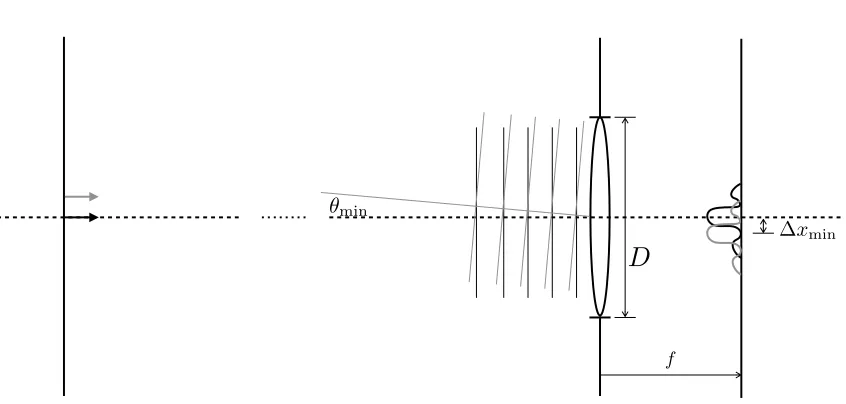
As was previously mentioned, the GIQE indicates that the resolution of an imaging system is the dominant predictor of the ultimate quality of its images. While resolution in the GIQE is measured in terms of ground sample distance, the true nature of resolu-tion is more complex and must be understood when analyzing systems with non-circular apertures. Under the Rayleigh resolution criterion, resolution is defined in terms of two identical point sources. As these point sources are brought closer together, there will come a point at which they will be indistinguishable from a brighter, single point source positioned directly between the two point sources. This situation is illustrated in Figure 1.1. The distance between these two point sources at which this confusion occurs is the resolution limit of that system. The Rayleigh criterion states that this resolution limit is directly determined by the size of the point spread function (PSF) of the imaging system, or the amount of blur it introduces [Goodman, 2005]. The size of the system’s PSF can be determined by a large number of parameters; some of these parameters are controllable by the designer of the imaging system, while others are unavoidable.

(19)

5

✓min

f

D

[image:19.612.129.552.116.318.2]

xmin

Figure 1.1: An illustration of the Rayleigh resolution criterion

limited by diffraction. Other factors, such as optical aberrations, detector sampling rates and atmospheric scattering, may also be limiting factors in imaging resolution. However, in the absence of all other factors, the conventional imaging system can never hope to achieve resolution greater than the diffraction limit for a single exposure. For an imaging system with a circular aperture function, the angular resolution limit of incoherent incident radiance due to diffraction is given by

θmin= 1.22

λ

D [radians] (1.2)

whereλis the wavelength of the light being imaged andDis the diameter of the aperture

of the imaging system. For applications that are imaging on a focal plane, this expression can be reformulated to give the resolution in terms of distance on the focal plane. This is

done by using the focal length,f, of the system,

∆xmin= 1.22

λf

D = 1.22λ(F#) [m] (1.3)

whereF# = f /Dis the F-number of the system. Examining these equations yields

(20)

res-6

olution than a system with a smaller aperture. Given that resolution has been determined to be the dominant factor in image quality, it also stands to reason that the larger system will have better image quality, assuming the other terms in the GIQE can be held constant.

Practically speaking, holding focal length constant while increasing the diameter leads to a surface with increased thickness and sag. This often leads to an increase in the amount of optical aberration present in the optics, which can degrade image quality. In addition to an increase in aberration, larger apertures also come at the expense of the overall weight, volume and cost of the imaging system. For a traditional system, the cost tends to scale by at least the square of the diameter [AWMA and SPIE, 1996] While this is a problem for ground-based imaging systems, it is a prohibitive issue for space-based imaging systems, as launch vehicles can only take a given amount of mass and volume into space. Thus, until optics for space-based imaging systems can be fabricated and assembled in space, imaging systems will have to operate under a mass and volume constraint. This gives rise to the challenge of balancing the resolution of space-based systems against the mass and volume of the system. Ignoring the enclosures, electronics and other satellite components, this challenge is equivalent to maximizing the amount of resolution obtained from a given amount of glass or volume.

(21)

Chapter 2

Objectives

This chapter will outline the top-level objectives of this research and indicate the contri-butions of these objectives. As was mentioned in Chapter 1, this research will focus on the problem of sparse aperture image quality, specifically in a remote sensing situation. That is, the sparse aperture system will be focused at infinity and the input to the system will be polychromatic incoherent illumination. Given this imaging situation, the research proposed here will focus on two main efforts. The first of these is to perform a labora-tory validation study of the sparse aperture system modeling methodology summarized in Chapter 4. Validation of monochromatic sparse aperture point spread functions have been attempted before, however, this research will aim to build upon previous studies. The main components of this research are:

• Design a laboratory optical system that can be used to simulate a sparse aperture

system. This system should be able to:

– Simulate a system with negligible wavefront error.

– Introduce small amount of wavefront error in a characterizable manner

– Provide controllable or characterizable broadband illumination to the imaging

system.

– Provide a mechanism by which to measure the system modulation transfer

function.

– Provide a mechanism by which extended scene analysis may be performed.

• Construct the designed laboratory system.

(22)

8

• Perform validation experiments on a sparse aperture system that can be replicated

in the computer model.

– Isolate the MTF contributions due to the aberrated pupil function.

– Verify the predicted existence of post processing artifacts in observed imagery.

This validation study offers a number of advantages over existing studies. Previous studies have focused on measuring the monochromatic point spread function of a sparse aperture system. This study will also allow for the inclusion of spectral effects and wavefront error. This will allow a system designer to greater explore a larger portion of the sparse aperture design space using a validated model. The OTF validation experiment will be described in Chapter 5. In addition, this system will allow for the introduction of extended scenes into the system. Simulation of sparse aperture imagery in previous studies has indicated the possibility of unpleasant image artifacts due to post-processing. This research will allow for the verification of these artifacts in real imagery. The methods and results of this study will be presented in Chapter 6.

Once the modeling methodology has been validated, it can be used to predict the performance of theoretical sparse aperture systems. Thus, it can be a useful tool in trade studies involving sparse aperture system design. For example, if reconnaissance applications are being targeted, a ∆NIIRS study, like the one presented in [Garma, 2015], could be performed with the model’s imagery predictions. Alternatively, if an automated analysis, such as crop coverage classification, is the targeted application, modeled imagery can be used as test data to assess the performance of a proposed telescope design. In this research, two design problems will be investigated: subaperture layout and spectral bandpass selection. These studies will both serve as demonstrations of how the validated model can be used to aid in design studies. However, because sparse aperture image quality is not yet a well-understood problem, these demonstrations are intended as starting points, and not as authoritative conclusions on optimal sparse aperture system design. The main components of this research are:

• Create a subaperture layout optimization algorithm.

• Validate the functionality of the algorithm by replicating previous work in sparse

(23)

9

• Use the layout optimization algorithm to design apertures that overcome or are more

resistant to the issues present in sparse aperture remote sensing systems. These include:

– The anisotropic nature of sparse aperture optical transfer functions.

– The presence of ringing artifacts as a result of post-processing filters.

• Identify the effects of spectral knowledge on sparse aperture image quality after

post-processing.

• Analyze the effects of narrow bandpass designs and broad bandpass designs on image

quality under different spectral knowledge levels.

• Design and execute a laboratory experiment to validate expected spectral behavior

in a simple imaging scenario.

(24)

Chapter 3

Background

This chapter will lay out the theory behind the prediction of the performance of imaging systems with non-conventional aperture functions. In order to fully understand the mod-eling of these systems, theory will be presented on the majority of the imaging chain. The main differences for non-conventional aperture systems are confined to light acquisition and image processing. However, a full knowledge of the imaging chain is necessary to construct an accurate image quality model. A reader interested in further imaging chain analysis in the context of remote sensing is referred to [Schott, 2007].

The theoretical modeling approach taken will rely heavily on the linear systems theory for image formation [Gaskill, 1978]. This approach allows for the use of convolution to model the degradation of imagery due to diffraction, aberrations and image motion. This framework also allows for the introduction of noise into the system and the derivation of the linear filters to apply in post-processing image enhancement. Aberration theory is also necessary to understand the various effects other than diffraction that can degrade image quality. The radiometry associated with such an imaging system will also be introduced.

(25)

3.1. LINEAR SYSTEMS IN IMAGING 11

3.1

Linear Systems in Imaging

Original Input Original Output

Scaled and Shifted Input Scaled and Shifted Output

O

Figure 3.1: Illustration of linearity and shift invariance

Under the common assumption that an imaging system is both linear and shift invariant, linear systems theory may be used to predict the performance of that system. If we assume

that the imaging process is some operator,_O, then the process is linear if

O{a·f1[x, y] +b·f2[x, y]}=a· O{f1[x, y]}+b· O{f2[x, y]} (3.1)

where a and b are scalars and fn[x, y] is an input to the imaging system. The imaging

operatorO is said to be shift invariant if

g[x, y] =O{f[x, y]} =⇒ g[x−x0, y−y0] =O{f[x−x0, y−y0]}

wherex0 and y0 are scalar constants. This property is illustrated in Figure 3.1. As shall

be seen later, the assumption of linearity and shift invariance is normally invalid across the entire image plane, however, it can be made over small portions of the image plane and thus linear systems theory can be used in a piecewise manner over the image plane to predict the performance of an imaging system.

(26)

3.1. LINEAR SYSTEMS IN IMAGING 12

may be characterized as a convolution. If the input to the system is a point source of light, represented as a Dirac delta function, then the output predicted by the convolution will be the convolution kernel for the imaging system,h[x, y]. Since this kernel describes the image of a point source, it is termed the Point Spread Function (PSF) of the imaging system. The performance of the imaging system is then characterized in an LSI region by

g[x, y] =

∞ Z −∞ ∞ Z −∞

h[α, β]·f[x−α, y−β]dα dβ (3.2)

= f[x, y]∗h[x, y] (3.3)

When dealing with imaging system modeling, these convolutions are often computed in

the frequency domain through the use of the Fourier transform operator,_F, defined as

F[ξ, η] =_{F {}f[x, y]_}=

∞ Z −∞ ∞ Z −∞

f[x, y]e−2πi(ξx+ηy) dx dy (3.4)

The advantage of utilizing the frequency domain is that convolutions, which are computa-tionally expensive to evaluate in the spatial domain, can be evaluated as simple element-wise multiplications in the frequency domain, due to the Fourier convolution theorem [Easton, 2010]. Thus,

g[x, y] =f[x, y]_∗h[x, y] =_F−1_{{F {}_f_[_{x, y}_]_{} · F {}_h_[_{x, y}_]_}} _(3.5)

where_F−1 _{is the inverse Fourier transform, defined as}

f[x, y] =F−1_{_F_[_{ξ, η}_]_}₌

∞ Z −∞ ∞ Z −∞

F[ξ, η]e+2πi(ξx+ηy) dξ dη (3.6)

This property is useful due to the existence of the Fast Fourier Transform (FFT), an algo-rithm to evaluate the Fourier transform inO(nlogn), or log-linear, time. Since evaluating the two forward and one inverse transform all take log-linear time and the element-wise multiplication is a O(n), or linear time, operation, the entire evaluation is a log-linear,

O(nlogn), computation, wherenis the number of pixels in the image. On the other hand,

(27)

3.1. LINEAR SYSTEMS IN IMAGING 13

shifted to be centered at every element of the other array and the two then need to be

multiplied and summed at every shift. This results in a quadratic, O(n2_{), time process.}

Thus, for reasonably large arrays, the frequency domain evaluation will be more efficient than the spatial domain evaluation. An example of this tradeoff is given in Figure 3.2.

0 50 100 150 200 250 300 350 400 450

2 4 6 8 10 12 14 16 18 20

Computation Time

n

O(n2) O(n log n)

Figure 3.2: Example of the computation time curves forO(nlogn) vs O(n2_{) algorithms.}

Precise values ofnand computation time depend on the implementation.

Given the Fourier transform and the convolution theorem, the imaging relationship given in Equation 3.3 can be re-expressed as

G[ξ, η] =F[ξ, η]·H[ξ, η] (3.7)

whereH[ξ, η] is the Fourier transform of the system’s PSF. This term is commonly referred to as the Optical Transfer Function (OTF) of the imaging system. This formulation of the imaging problem is highly advantageous for imaging system modeling when using the Imaging Chain approach.

(28)

3.2. THE IMAGING CHAIN APPROACH 14

of the system. Linear systems theory often makes the simplifying assumption that noise is additive and independent of the signal, so that Equation 3.7 may be rewritten as

G[ξ, η] =F[ξ, η]_·H[ξ, η] +N[ξ, η] (3.8)

While this assumption is invalid due to photon noise, it is only utilized when deriving a linear image restoration filter, as will be discussed later. As a result, the final image quality is sub-optimal due to this assumption and a better, non-linear, restoration procedure may exist.

3.2

The Imaging Chain Approach

As seen in Figure 3.3, the Imaging Chain approach looks at the imaging process as a series of steps. The process begins at the light source and then considers interactions with the object of interest and its surroundings. Light then continues to interact with the environ-ment until some of it reaches the imaging system’s light collection apparatus. Once light is collected, it must be detected by the imaging system and converted into a measurable signal. This signal is then processed to produce a final image. This final image may then be displayed and perceived by an end user or automatically analyzed by a computer.

Source Object Collection Detection Processing

Display Perception

Analysis

Figure 3.3: The Imaging Chain approach breaks down the imaging process into a series of links with limited interactions.

(29)

3.3. PROPAGATION OF LIGHT TO THE ENTRANCE PUPIL 15

Modern digital detectors have a pixel footprint, or a rectangular region over which photons are integrated. This is a blurring and sampling function of the light distribution that was imaged onto the detector and thus a signal degradation. Once images are captured, image enhancement algorithms are performed on the image, again changing the signal, although ideally not a degradation. The Imaging Chain approach ties nicely into the linear systems approach described in the previous section if linear shift invariant assumptions are made on each of the steps. In this case,

G[ξ, η] = Y

i

Hi[ξ, η] !

·F[ξ, η] (3.9)

whereHi[ξ, η] is the OTF produced by each step in the imaging process. Note that each

link in the imaging chain is complex and can contain multiple steps.

Since light-object interactions are invariant with respect to the design of passive imag-ing systems, this research will be focusimag-ing on the light collection, detection and processimag-ing steps. Every optical component in an imaging system has the ability to degrade the sig-nal and thus each optical element has its own OTF. The detector also has an associated OTF. In addition to the sampling footprint, pixel crosstalk, or signal leakage, can further complicate the OTF of an imaging detector. Finally, signal post-processing, when done with linear filters, also have associated OTFs. The cascading of multiple OTFs, described in Equation 3.9, will be used extensively in the modeling of complex optical systems.

3.3

Propagation of Light to the Entrance Pupil

(30)

3.3. PROPAGATION OF LIGHT TO THE ENTRANCE PUPIL 16

that for a Lambertian object, this radiance distribution can be approximated as

L(λ) = Es,exo(λ) cosσ0τ1(λ)τ2(λ)

ρ(λ)

π +(λ)Lemis(λ, T)τ2(λ) +F Eds(λ)τ2(λ) ρ(λ)

π

+F Ede(λ)τ2(λ)

ρ(λ)

π + (1−F)[Lbs(λ) +Lbe(λ)]τ2(λ)ρ(λ)

+Lus(λ) +Lue(λ) (3.10)

In this equation, Es,exo represents the exoatmospheric solar irradiance, σ0 is the solar

angle with respect to the target,τ1 is the transmission from the top of the atmosphere to

the target, τ2 is the transmission from the target to the imaging system, ρ is the diffuse

target reflectance,is the target’s emissivity, Lemis is the blackbody radiance due to the

target’s temperature,T, F is the sky fraction of the hemisphere above the target, Eds is

the reflected downwelled irradiance, Ede is the emitted downwelled irradiance, Lbs is the

average radiance reflected by non-sky background,Lbeis the average emitted radiance from

non-sky background, Lus is reflected upwelled radiance and Lue is the emitted upwelled

radiance.

Es,exo

⌧1

0

F Eds

⌧2 Lus

L

Lbs

Figure 3.4: Illustration of the components of reflected sensor-reaching radiance.

(31)

3.4. DIFFRACTION-LIMITED IMAGING 17

shortwave infrared spectral regions, thermal emission is negligible, yielding,

L(λ) = Es,exo(λ) cosσ0τ1(λ) +F Eds(λ)

ρ(λ)τ2(λ)

π

+(1₋F)Lbsτ2(λ)ρ(λ) +Lus (3.11)

The components of this equation are visualized in Figure 3.4. In these equations, the transmission terms, downwelled irradiance and upwelled radiance are all atmospheric terms that need to be modeled. Traditionally, this is done using an atmospheric models, such as MODTRAN [Berk et al., 1989]. The sky fraction and average background radiance terms depend on the scene structure around the target. The radiance field reaching the front of the system predicted by Equation 3.11, represents the ideal image that can be obtained through the imaging system. Given that no imaging system can perfectly replicate this radiance field, the degration effects of the optical system on image quality must now be examined.

3.4

Diffraction-Limited Imaging

z

E(x, y,0) E(x, y, z)E0_{(x, y, z)} _E₍_{x, y, z}₊_f₎

f

p(x, y)

(32)

3.4. DIFFRACTION-LIMITED IMAGING 18

As was alluded to in the Imaging Chain section, each optical element in a system will degrade the quality of the image. Every optical component, even one made perfectly to specification, will degrade the signal due to the fact that it has a finite size. The finite size of the optic results in diffraction effects, which blur the light distribution. An optic which degrades the signal primarily due to its diffraction effects and not any imperfections in the optic itself is termed diffraction-limited. To see the effects of this, an example of a finite lens with perfect focusing ability will be examined. This is shown in Figure 3.5. In this figure, the light distribution at the object plane, z= 0, is shown as an off-axis point

source, the light then propagates over a long distancezto the lens. As derived in [Easton,

2010], Fresnel diffraction is used to propagate the light to the lens and from the lens to the image plane. The aperture function attenuates the wavefront at the aperture plane. The expression for the final electric field at the image plane is actually a convolution with the input signal, where the impulse response is given by,

ˆ h

"

x, y;z1 =

1

f −

1 z0

−1#

∝P x λz1 , y λz1 (3.12)

whereP is the Fourier transform of the pupil function. This is an important observation;

in the absence of all other aberrations, the degradation in image quality by an optic is determined by the shape of the aperture function. However, this expression operates on the electric field of the light, which is not directly measurable by modern imaging detectors. Instead these detectors measure exposure, i.e. irradiance integrated over a finite time interval. Irradiance is defined as the time average of the squared magnitude of the electric field. So, in this case, the PSF due to diffraction, normalized to unit area, is given by

h

"

x, y;z1 =

1

f −

1 z0

−1#

= 1 k P x λz1 , y λz1 2 (3.13) k = ∞ ZZ −∞ P x λz1 , y λz1 2

dx dy (3.14)

The OTF due to diffraction is then given by

H

"

ξ, η;z1=

1

f −

1 z0

−1#

= 1

(33)

3.4. DIFFRACTION-LIMITED IMAGING 19

where the F operator signifies the autocorrelation operation and p is the spatial domain

pupil function.

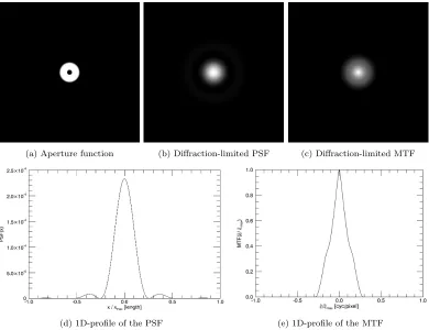
(a) Aperture function (b) Diffraction-limited PSF (c) Diffraction-limited MTF

[image:33.612.145.535.192.495.2]

(d) 1D-profile of the PSF (e) 1D-profile of the MTF

Figure 3.6: Diffraction-limited imaging performance of a circular aperture.

3.4.1 Symmetric Aperture Functions

(34)

3.4. DIFFRACTION-LIMITED IMAGING 20

While the circular aperture is a simple case, it is not always practical to build space-based telescopes with a circular aperture. Many of these telescopes instead have a sec-ondary focusing mirror that blocks the central portion of the primary mirror, as occurs in the Cassegrain design, shown in Figure 3.7. Since the secondary mirror blocks some rays from entering the system, it introduces a central obscuration into the aperture func-tion. This obscuration has little effect on the low- or high-frequency values of the MTF, however, it does cause a dip in the mid-frequency response of the system. In the spatial domain, the peak of the PSF has been reduced in magnitude. More energy is also in the secondary peaks than in the case of the unobstructed circular aperture. These effects can be seen in Figure 3.8.

(35)

3.4. DIFFRACTION-LIMITED IMAGING 21

(a) Aperture function (b) Diffraction-limited PSF (c) Diffraction-limited MTF

[image:35.612.144.534.133.433.2]

(d) 1D-profile of the PSF (e) 1D-profile of the MTF

Figure 3.8: Diffraction-limited imaging performance of an obstructed circular aperture.

3.4.2 Non-symmetric Aperture Functions

(36)

3.4. DIFFRACTION-LIMITED IMAGING 22

(a) Aperture function (b) Diffraction-limited PSF (c) Diffraction-limited MTF (contrast-stretched)

Figure 3.9: Diffraction-limited imaging performance of a Tri-arm 9 design.

(a) Aperture function (b) Diffraction-limited PSF (c) Diffraction-limited MTF (contrast-stretched)

Figure 3.10: Diffraction-limited imaging performance of a Golay-6 design.

(37)

3.5. ABERRATION THEORY 23

property of the Dirac delta function can be used to reformulate the pupil function,

p[x, y] =

N X

i=1

psub[x−xi, y−yi] (3.16)

= psub[x, y]∗

N X

i=1

δ[x−xi, y−yi] (3.17)

where psub is the aperture function of the sub-aperture, (xi, yi) is the center position of

the ith sub-aperture and N is 9 in this case. The diffraction limited OTF is then given

by equation 3.15.

OT F = 1

kpsub[−λz1ξ,−λz1η]∗

N X

i=1

δ[−λz1ξ−xi,−λz1η−yi]∗

p∗_sub[₋λz1ξ,−λz1η]∗

N X

i=1

δ[₋λz1ξ+xi,−λz1η+yi]

= 1

k(psub[−λz1ξ,−λz1η]Fpsub[−λz1ξ,−λz1η])∗

N X i=1 N X j=1

δ[−λz1ξ−xi+xj,−λz1η−yi+yj] (3.18)

This result shows that the diffraction-limited OTF of a sparse aperture design, composed of identical sub-apertures, is given by the sum of shifted copies of the diffraction-limited OTFs of the sub-apertures, which is why sparse aperture OTFs often exhibit secondary peaks.

3.5

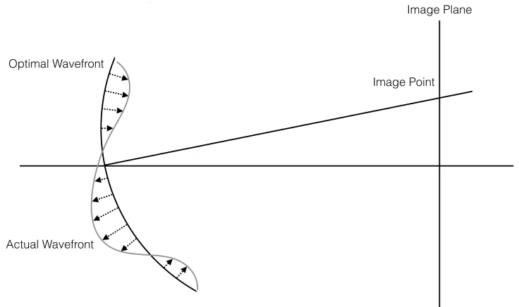
Aberration Theory

(38)

3.5. ABERRATION THEORY 24

Image Point Image Plane

Optimal Wavefront

[image:38.612.155.523.133.351.2]

Actual Wavefront

Figure 3.11: Deviations from a spherical wavefront result in aberrations

In the case of perfect imagery, the wavefront error is zero for all points along the wave-front. However, wavefront error tends to be non-zero and gets larger as the distance away from the optical axis increases. Just as the radiance field entering an optical system is a four-dimensional function, the wavefront aberration function is also four-dimensional. That is, it depends on both the two-dimensional coordinates on the aperture and the incoming direction. Equivalently, if there is a defined object plane, wavefront aberration depends on both aperture coordinates and object coordinates. This is illustrated with a sample aperture in Figure 3.12.

In the case of a circularly symmetric system, the dimensionality can be reduced by one. Since the aperture is circularly symmetric, the aberration is constant with respect to object orientation, so only the case of an axis-aligned object needs to be considered. Then, due to the symmetry, the aberration is dependent on the radius in aperture space,

ρand the cosine of the angle from the object’s axis to the ray intersection on the aperture

plane, cosφ. Under these conditions, aberration can only take on a limited number of

(39)

3.5. ABERRATION THEORY 25

(x, y)

(x0_{, y}0₎

Figure 3.12: Wavefront aberration is a four-dimensional function, depending on the in-coming ray direction and intersection coordinates on the aperture

The wavefront aberration function represents the change in optical path length based on the entrance location and angle of the optical path through the optical system. So, the aperture function can be re-expressed at a given object plane location, as

p[x, y, x0, y0] =|p[x, y, x0, y0]|e2πiW(x,y,x0,y0) (3.19) where_|p[x, y, x0_{, y}0_]_|_{is the mask of the aperture, generally a binary “zero-and-one” function}

(40)

3.6. PROPAGATION OF LIGHT TO THE SENSOR 26

Spherical

Tilt X

Tilt Y

Defocus

Coma X

Coma Y

Astigmatism 0/90

Astigmatism 45

Figure 3.13: Example instantiations of wavefront aberrations. Brightness is proportional to optical path length error.

OTF, termed isoplanatic regions.

Table 3.1: Aberrations for circularly symmetric optical systems

Aberration Wavefront ErrorW(h, ρ,cosφ)

Piston Error W000, W200h2, W400h4

Defocus W020ρ2

Tilt W111hρcosφ

Spherical W040ρ4

Coma W131hρ3cosφ

Astigmatism W222h2cos2φ

Field Curvature W220h2ρ2

Distortion W311h3ρcosφ

3.6

Propagation of Light to the Sensor

(41)

3.6. PROPAGATION OF LIGHT TO THE SENSOR 27

As the previous sections have stated, there is a blurring effect that occurs between the entrance pupil and the exit pupil. In an isoplanatic region, this blurring can be evaluated as a convolution. In order to convert radiance reaching the exit pupil to irradiance on the

detector, the G-Number (G#) is used.

G#(λ) = 1 + 4(f /#)

2

πF τ(λ) (3.20)

where f /# is the system F-Number, F is the system’s fill factor, or the fraction of the

pupil area that is transmissive, andτ is the transmission spectrum of the optics. The fill

factor term is normally omitted in systems with circular apertures as it is equal to one, however, it must be included in systems with sparse apertures. The spectral irradiance on the detector in an isoplanatic region is then given as,

Edet(x, y, λ) =

Lsource(x, y, λ)∗h(x, y, λ)

G# (3.21)

whereh(x, y, λ) is the point spread function given as the inverse Fourier transform of the OTF given in Equation 3.15. It should be noted that while it is not explicitly noted in the

equations,Lsource and thus Edetare random variables, due to photon noise. That is, they

are actually Poisson variables, where the predicted radiometric value is both the mean and variance.

If it is assumed that the detector acts linearly at the input signal level, then the signal in volts for a given pixel on the detector is given as

Svolt(x, y) =Adtint

Z ∞

0

Edet(x, y, λ)R(λ) dλ+N(x, y) (3.22)

whereAd is the area of the pixel, tint is the integration time of the detector and R(λ) is

the responsivity spectrum of the detector and N(x, y) is the noise added by the

detec-tor. N(x, y) consists of all detector-generated noise sources, including dark current and

(42)

3.7. IMAGE ENHANCEMENT 28

3.7

Image Enhancement

As was seen in Figure 3.9, a sparse aperture function can result in an OTF that has support, i.e. energy, over a wide range of frequencies, even if the magnitude at those frequencies is relatively low. If the noise in the system is also relatively low, then the images produced by these systems are good candidates for image enhancement. Inverse filtering is the operation of trying to undo the process of a convolution, retrieving the input signal. Using an additive noise model and a convolution to model image degradation, the output image spectrum is given by

G[ξ, η] =F[ξ, η]·H[ξ, η] +N[ξ, η] (3.23)

The goal of inverse filtering is to recover F as closely as possible. Since noise is

un-known and convolution is almost always a non-invertible operator, the problem must be approached as a minimization of some error between the original object and the recon-structed image. A common error metric is the sum of the squared error. That is, the reconstructed image, ˆf, satisfies

argmin

ˆ

f N X

y=1

M X

x=1

(f[x, y]−fˆ[x, y])2 (3.24)

This problem is complicated by the fact that in an imaging situation, neither the object nor its spectrum is known. However, it can be shown that, given the assumption that the noise and signal are statistically independent, the minimum squared error can be minimized by the following filter function, known as the Wiener filter. [Easton, 2010]

W[ξ, η] = 1 H[ξ, η]

|F[ξ, η]|2

|F[ξ, η]_|2₊_|_N_[_{ξ, η}_]_|2 (3.25)

This equation can then be re-expressed in its more common form

W[ξ, η] = H

∗_[_{ξ, η}_]

|H[ξ, η]_|2₊|N[ξ,η]|2

|F[ξ,η]|2

(3.26)

(43)

3.7. IMAGE ENHANCEMENT 29

the denominator. The effect of this term is to make the filter act as an inverse filter at frequencies where the signal-to-noise ratio is high and as a noise suppressor at frequencies where the signal-to-noise ratio is low. This overcomes the primary downfall of the naive inverse filter, which is the boosting of noise at spatial frequencies with low signal-to-noise ratios.

0 0.2 0.4 0.6 0.8 1

0 0.1 0.2 0.3 0.4 0.5 0

5 10 15 20 25

MTF

Restoration Filter

Spatial Frequency [cyc/pixel] MTF Inverse Filter Wiener Filter

Figure 3.14: An example of a Wiener filter with a constant noise spectrum

As can be seen in Equation 3.26, the transfer function in the numerator is a complex function. This is advantageous as the transfer function of optical systems is often complex due to wavefront aberrations. If these wavefront aberrations have been characterized for a system, the system’s complex transfer function can be input into the Wiener filter in order to compensate for these aberrations. This can be very useful in the case of sparse aperture systems. Small aberrations can result in the disappearance of some of the peaks in the system’s OTF. Using the unaberrated OTF in the Wiener filter would result in inverse filtering at these frequencies. Since the aberrations eliminated the signal at those frequencies, the unaberrated Wiener filter would simply boost noise and introduce ringing artifacts, degrading the resulting image.

(44)

ap-3.7. IMAGE ENHANCEMENT 30

(a)γ= 0.1 (b)γ= 0.01 (c)γ= 0.001

Figure 3.15: Examples of constrained least-squares restoration filters for a circular

aper-ture. Notice that as γ decreases, higher frequencies are increasingly boosted.

proximated, the output image spectrum can be used as an approximation of the object spectrum. The filter can then be iterated, updating the image spectrum after each itera-tion. This is known as the iterative Wiener-Helstrom filter [Schott, 2007]. Another option is to simply use a constant value for the noise-to-singal term. The option used in this research was a constrained least-squares variant of the Wiener filter. [Reddi, 1978]

ˆ

F[ξ, η] =W[ξ, η]·G[ξ, η] = H

∗_[_{ξ, η}_]

|H[ξ, η]_|2₊_γ_{· |}_S_[_{ξ, η}_]_|2 ·G[ξ, η] (3.27)

Instead of simply using a constant in the denominator, a local image smoothness term

is added to the denominator. This term S[ξ, η] is the transfer function of a Laplacian

convolution kernel. This term is modulated by a tunable scalar, γ that can be used to

adjust the amount of inverse filtering or blurring that occurs as a result of the filter. The effect of this parameter on the restoration filter is shown in Figure 3.15. Optimal determination of this parameter is difficult, but depends on the noise present in the output

image and the use case of the output image. For instance, the value ofγ that is optimal

for human perception at a given noise level might differ from the optimal value of γ if

the image were to be used for some automated processing. In practice, the value of γ is

empirically tuned for the given imagery to give an optimal output. For low noise inputs,

γ tends to be less than one. As γ increases beyond one, the inverse filter becomes more

(45)

Chapter 4

Modeling Approach

DIRSIG Scene Radiance

⇥ F{·}

Binary Pattern   with Known Illumination

Isoplanatic Regions

Aperture Mask Wavefront Error Aberrated Optics OTF

Isoplanatic Interpolation

Blurred Sensor- Reaching Irradiance

Detector Sampling OTF Jitter OTF Smear OTF

⇥ ⇥ ⇥

F 1

{|F{·}|2

}

Figure 4.1: A flowchart visualization of the modeling approach to produce raw sensor-reaching irradiance.

This chapter will explain the approach taken to model optical systems with non-conventional aperture functions, applying the theory presented in the previous chapter. A graphical overview of the first half of the model is given in Figure 4.1. In this figure, the process

(46)

32

of obtaining the irradiance field incident on the detector is shown. The process by which this is converted into a final image is illustrated in Figure 4.2.

Aperture Mask Wavefront Error Estimate

Blurred Sensor-Reaching Signal

R( )

X

{·}

Detector Noise

+

Detected Image

⇥

F{·}

Inverse Filter

Restored Image Isoplanatic

Interpolation

Isoplanatic Regions

Figure 4.2: A flowchart visualization of the modeling approach to produce a final restored image.

(47)

4.1. PREVIOUS WORK 33

and smear due to linear motion over the integration time, all of which are assumed to be constant over the spectral dimension.

Once degraded, the signal is spectrally summed over the bandpass(es) of the detector and degraded by the addition of detector noise, giving an approximation of Equation 3.22, or the raw image that was detected by the imaging system. This image is then processed by a restoration filter to produce the final restored image. This restoration filter is produced from knowledge of the aperture shape and an approximation of the wavefront error across the aperture, as it may be impractical to precisely measure this error once the system has been deployed. This inverse filtering can also be applied in a spatially-varying manner, if off-axis aberration in the system can be characterized.

4.1

Previous Work

Sparse aperture arrays have had a long history in both radio astronomy, infrared astron-omy and optical physics. In 1970, a sparse aperture telescope for use in the long-wave infrared was being designed by [Meinel, 1970]. The problem of layout optimization also has a long history, with [Golay, 1971] designing aperture configurations to give desirable MTF characteristics. More recently, research has picked up into modeling and creating sparse aperture telescopes for remote sensing purposes. Unlike previous research into the topic, the area of interest here is in the visible to near-infrared region of the electromag-netic spectrum. This is a more challenging problem, as alignment tolerances scale with wavelength, resulting in the need for optical systems with an extreme amount of precision. [Fiete et al., 2002] from the Eastman Kodak Company have performed a number of image quality studies exploring the trade spaces of sparse aperture design. Confining analysis to three well-known sparse aperture designs (Tri-arm 9, Golay 6 and annulus), their work analyzed the tradeoff of fill factor and integration time, finding that integration time had

to be increased by a factor in the range of 1/F2 _{to 1}_/F3_{, depending on aperture design.}

This conclusion agreed with the conclusion of [Fienup, 2000], who found the 1/F3 _factor

(48)

4.1. PREVIOUS WORK 34

[Breckinridge et al., 2008] built upon this work even further, looking at more optical designs and low-contrast imaging situations. In such situations, they found the exponent in the integration time versus fill factor tradeoff could reach 4 or 5 depending on contrast level and subaperture layout. The large effects of signal-to-noise ratio on the imaging parameters of sparse aperture systems in this work also strengthen the argument against using GIQE for sparse aperture imagery. In the GIQE, SNR is weighted relatively lightly compared to spatial resolution and the SNR levels of the conventional imagery used to fit the GIQE were obtained with a much shorter integration times than would be required in a sparse system.

The model outlined in the chapter introduction is the result of several research projects. The original model was introduced by [Introne et al., 2005]. In this work, the three well-known sparse aperture designs from [Fiete et al., 2002] were extensively analyzed using the modeling approach. This work also established the importance of using polychromatic simulation in sparse aperture modeling, showing that a grey-world assumption was not sufficient for image quality studies with these systems. This work was extended by [Block, 2005], who examined the spectral issues of sparse aperture imaging in more detail. This work conducted a sensitivity study to examine the nature of spectral artifacts that arise due to inverse filtering in a panchromatic system. The findings of these works are the primary focus of the validation study proposed in this research.

(49)

4.2. RADIANCE IMAGE 35

apertures by [Smith, 2012]. In this work, target detection was used as the benchmark algorithm with comparative analysis performed on monolithic, Tri-arm 9 and hexagonal synthetic apertures.

All of the above works were confined to computer modeling of sparse aperture perfor-mance. [Chung et al., 2002] from the Massachusetts Institute of Technology have built a ground-based three-element sparse aperture telescope, called ARGOS. They have pub-lished an analysis of how the PSF degrades with alignment error and a cost analysis. Unfortunately, the cost of the system is in the hundreds of thousands of dollars, making their design impractical for a laboratory model validation study as proposed here. Ad-ditionally, no images from the telescope have been published. [Zhou et al., 2009] from Beijing University of Technology have constructed a low-cost laboratory setup utilizing masks to simulate sparse apertures. This setup is the one from which the setup in this research draws the most inspiration. Their setup utilizes refractive lenses (and thus has a limited spectral range) and has limited control over wavefront error, two factors this work will attempt to improve upon. Additionally, their study did not perform quantitative com-parison to modeled PSF/OTFs and was limited to the three well-known configurations. This works aims to expand upon both of these areas.

4.2

Radiance Image

As was described in Section 3.3, there are many terms that contribute to the radiance distribution that reaches the entrance pupil of an imaging system. In a remote sensing application, one has to consider direct solar illumination, diffuse illumination from the sky and energy scattered into the line of sight, amongst other terms. If infrared radiation is being examined, emitted radiation must also be considered. In order to model how a potential system will perform, realistic synthetic imagery needs to be generated using the theory presented.

(50)

near-4.2. RADIANCE IMAGE 36

530 nm

810 nm

Figure 4.3: Sample bands of a DIRSIG-generated hyper spectral input to the model

infrared spectrum in this research. In order to produce high-fidelity images, the model needs to incorporate a lot of information about the scene. Some of these inputs include spectrally-attributed scene geometry, atmospheric conditions, scene thermal information and weather history. The technical details and intricacies of the model are out of the scope of this research, however, an interested reader is referred to the DIRSIG documentation (http://www.dirsig.org/docs/new/) for more details. In this research, the role of DIRSIG is to model the radiance distribution at the entrance pupil of the imaging system that we

wish to model, that is, it is providing the Lsource(x, y, λ) term in Equation 3.21. Some

example bands from a DIRSIG scene are given in Figure 4.3.

The radiance image,Lsource(x, y, λ), that is modeled by DIRSIG is a three-dimensional

data source. It has two spatial dimensions and one spectral dimension, similar to a hy-perspectral data cube. The model can be set up to vary the resolutions in all three of these dimensions. Since the DIRSIG model already performs spatial integration inside of a pixel through the use of adaptive sampling, the spatial resolution can be set to the size of the detector without any worry of introducing aliasing into the system, provided sufficient spatial oversampling was specified when generating the scene.

(51)

en-4.2. RADIANCE IMAGE 37

(a) Center: 550 [nm], FWHM: 1.5 [nm] (b) Center: 550 [nm], FWHM: 150 [nm]

Figure 4.4: Illustration of the effects of wavelength on the diffraction-limited performance of a Tri-arm 9 sparse aperture design.

tire visible range, while hyperspectral systems can have bandpasses that span only a few nanometers. Thus, the spectral resolution of the input radiance image should be depen-dent on the bandpasses that are going to be modeled and should always be higher than the bands being modeled. As was shown in Equation 3.15, the optical transfer function due to diffraction is highly dependent on wavelength. As such, the degradation of the signal can vary significantly over a panchromatic or multispectral band. This effect is illustrated in Figure 4.4 for a Tri-arm 9 sparse aperture for a band centered around 550 nanometers with a full-width, half-max (FWHM) of 150 nanometers in comparison to the same band with a FWHM of 1.5 nanometers.

(52)

4.3. ABERRATED OPTICS OTF 38

4.3

Aberrated Optics OTF

Under normal operating conditions, the optics of a sparse aperture system provide the pri-mary degradation of image quality. As such, the modeling approach for this degradation should be as accurate as possible. The inputs to the model that facilitate this model-ing are the aperture mask that defines the unaberrated pupil function and the wavefront error at each point on the aperture. These inputs are given as two-dimensional images. This representation carries some inherent assumptions. As was illustrated in Figure 3.12, wavefront error is a four-dimensional quantity. The aperture mask is representative of the transmission through the optics along every optical path, which is also four-dimensional. Due to the large object distances present in remote sensing situations, the field of views of these systems tend to be very small. Thus, within an isoplanatic region of the image plane, the transmission and wavefront error are assumed to be constant with respect to incoming ray angle. This assumption is closely tied to that of local linearity and shift-invariance, allowing the computation of image degradation as a convolution.

Given the assumption that the aperture mask and wavefront error can be expressed as two-dimensional quantities, the complex pupil function can be expressed as

p[x, y] =_|p[x, y]_|e2πiW(x,y) _(4.1)

where _|p[x, y]_| is the aperture mask and W(x, y) is the wavefront error, in waves. Note

that there is an implicit spectral dependence here, as the waves unit on W(x, y) is given

in terms of some reference wavelength, λ0. The wavelength dependence is made explicit

below,

p[x, y, λ;λ0] =|p[x, y]|e2πiW(x,y) λ₀

λ (4.2)

(53)

4.3. ABERRATED OPTICS OTF 39

(a) Piston/tip/tilt wavefront error (b) Aberrated MTF: 0.1 waves RMS

[image:53.612.14

Image Quality Modeling and Optimization for Non-Conventional Aperture Imaging Systems

Rochester Institute of Technology

Recommended Citation

CHESTER F. CARLSON CENTER FOR IMAGING SCIENCE

Contents

List of Figures

Image Quality Modeling and Optimization for Non-Conventional

Chapter 1

Chapter 2

Chapter 3

3.1. LINEAR SYSTEMS IN IMAGING 11

Linear Systems in Imaging

3.1. LINEAR SYSTEMS IN IMAGING 12

3.1. LINEAR SYSTEMS IN IMAGING 13

3.2. THE IMAGING CHAIN APPROACH 14

The Imaging Chain Approach

3.3. PROPAGATION OF LIGHT TO THE ENTRANCE PUPIL 15

Propagation of Light to the Entrance Pupil

3.3. PROPAGATION OF LIGHT TO THE ENTRANCE PUPIL 16

3.4. DIFFRACTION-LIMITED IMAGING 17

Diffraction-Limited Imaging

3.4. DIFFRACTION-LIMITED IMAGING 18

3.4. DIFFRACTION-LIMITED IMAGING 19

3.4. DIFFRACTION-LIMITED IMAGING 21

3.5. ABERRATION THEORY 23

Aberration Theory

3.5. ABERRATION THEORY 24

3.5. ABERRATION THEORY 25

3.6. PROPAGATION OF LIGHT TO THE SENSOR 26

Spherical

Propagation of Light to the Sensor

3.6. PROPAGATION OF LIGHT TO THE SENSOR 27

3.7. IMAGE ENHANCEMENT 28

Image Enhancement

3.7. IMAGE ENHANCEMENT 29

Chapter 4

4.1. PREVIOUS WORK 33

Previous Work

4.1. PREVIOUS WORK 34

Radiance Image

4.3. ABERRATED OPTICS OTF 38

Aberrated Optics OTF

4.3. ABERRATED OPTICS OTF 39