Determination of a time-dependent thermal diffusivity and free boundary in heat conduction

This is a repository copy of Determination of a time-dependent thermal diffusivity and free

boundary in heat conduction.

White Rose Research Online URL for this paper:

http://eprints.whiterose.ac.uk/81062/

Version: Accepted Version

Article:

Hussein, MS and Lesnic, D (2014) Determination of a time-dependent thermal diffusivity

and free boundary in heat conduction. International Communications in Heat and Mass

Transfer, 53. 154 - 163. ISSN 0735-1933

https://doi.org/10.1016/j.icheatmasstransfer.2014.02.027

[email protected] https://eprints.whiterose.ac.uk/ Reuse

Unless indicated otherwise, fulltext items are protected by copyright with all rights reserved. The copyright exception in section 29 of the Copyright, Designs and Patents Act 1988 allows the making of a single copy solely for the purpose of non-commercial research or private study within the limits of fair dealing. The publisher or other rights-holder may allow further reproduction and re-use of this version - refer to the White Rose Research Online record for this item. Where records identify the publisher as the copyright holder, users can verify any specific terms of use on the publisher’s website.

Takedown

If you consider content in White Rose Research Online to be in breach of UK law, please notify us by

Determination of a time-dependent thermal diffusivity and free

boundary in heat conduction

M.S. Hussein1,2 _{and D. Lesnic}1

1_{Department of Applied Mathematics, University of Leeds, Leeds LS2 9JT, UK}

2_{Department of Mathematics, College of Science, University of Baghdad, Al-jaderia, Baghdad,}

Iraq

E-mails: [email protected] (M.S. Hussein), [email protected] (D. Lesnic).

Abstract

In this paper, we consider the inverse problem of simultaneous determination of time-dependent leading coefficient (thermal diffusivity) and free boundary in the one-dimensional time-dependent heat equation. The resulting inverse problem is recast as a nonlinear regularized least-squares problem. Stable and accurate numerical results are presented and discussed.

Keywords: Thermal diffusivity; Free boundary; Inverse problem; Heat equation.

1

Introduction

Many heat transfer applications can be modeled by the heat equation with a fixed boundary. However, there are numerous other problems for which the domain or the boundary varies with time and such problems are known as free boundary or Stefan problems [1]. For instance, when a conductor melts and the liquid is drained away as it appears, the heat conduction problem within the remaining solid involves the heat equation in a domain that is physically changing with time. In particular, the one-phase Stefan problem can be regarded as an inverse problem. In [2], the author investigated the heat equation with an unknown heat source in a domain with a known moving boundary. In [3, 4], the authors investigated the numerical solution of inverse Stefan problems using the method of fundamental solutions. In [5], an inverse moving boundary problem is solved using the least-squares method. In our work we consider the time-dependent nonlinear inverse one-dimensional and one-phase Stefan problem which consists in the simultaneous determination of the time-dependent thermal diffusivity and free boundary.

This paper is organized as follows: In the next section, we give the formulation of the inverse problem under investigation. The numerical methods for solving the direct and inverse problems are described in Sections 3 and 4, respectively. Furthermore, the numerical results and discussion are given in Section 5 and finally, conclusions are presented in Section 6.

2

Mathematical formulation

Consider the one-dimensional time-dependent heat equation

∂u

∂t(x, t) =a(t) ∂2u

∂x2(x, t) +f(x, t), (x, t)∈Ω (1)

in the domain Ω =_{(x, t) : 0< x < h(t),0< t < T <_∞}with unknown free smooth boundary

x=h(t)>0 and time-dependent thermal diffusivitya(t)>0. The initial condition is

u(x,0) =ϕ(x), 0_≤x_≤h(0) =:h0, (2)

whereh0 >0 is given, and the boundary and over-determination conditions are

u(0, t) =µ1(t), u(h(t), t) =µ2(t), 0≤t≤T, (3)

−a(t)ux(0, t) =µ3(t),

∫ h(t)

0

Note thatµ1 and µ3 represent Cauchy data at the boundary endx= 0, whilst µ4 represent the specification of the energy of the heat conducting system, [6].

First we perform the change of variable y = x/h(t) to reduce the problem (1)–(4) to the following inverse problem for the unknownsa(t), h(t) and v(y, t) :=u(yh(t), t):

∂v

∂t(y, t) = a(t)

h2_(t)

∂2_v

∂y2(y, t) +

yh′_(t) h(t)

∂v

∂y(y, t) +f(yh(t), t), (y, t)∈Q (5)

in the fixed domain Q = _{(y, t) : 0 < y < 1,0 < t < T_} with unknown time-dependent coefficientsa(t) and h(t). The initial condition is

v(y,0) =ϕ(h0y), 0≤y≤1, (6)

and the boundary and over-determination conditions are

v(0, t) =µ1(t), v(1, t) =µ2(t), 0_≤t_≤T, (7)

−a(t)vy(0, t) =µ3(t)h(t), h(t)

∫ 1

0

v(y, t)dy=µ4(t), 0≤t≤T. (8)

This model has been considered in [7]. The triplet (h(t), a(t), v(y, t)) is called a solution to the inverse problem (5)–(8) if it belongs to the class C1_{[0, T]×C[0, T]×C}2,1_{(Q), h(t) > 0,}

a(t)>0,t_∈[0, T], and satisfies the equations (5)–(8). For the input data we make the following regularity and compatibility assumptions:

(A) µi(t)∈C1[0, T],µi(t)>0 fort∈[0, T],i= 1,2,4,µ3(t)∈C1[0, T],µ3(t)<0 fort∈[0, T],

ϕ(x) _∈ C2[0, h0], ϕ(x) > 0, ϕ′(x) > 0 for x ∈ [0, h0], and f(x, t) ∈ C1,0([0, H1]×[0, T]),

f(x, t)_≥0 for (x, t)_∈[0, H1]×[0, T], where

H1 = max [0,T]µ4(t)

( min

{ min [0,h0]

ϕ(x),min

[0,T]µ1(t),min[0,T]µ2(t)

})−1

;

(B) ϕ(0) =µ1(0), ϕ(h0) =µ2(0), and∫h0

0 ϕ(x)dx=µ4(0).

The following existence and uniqueness of solution theorems are proved in [7].

Theorem 1. (Local existence)

If the conditions (A) and (B) are satisfied, then there exists t0 ∈ [0, T], (defined by the input

data) such that a solution of problem (5)–(8) exists locally for(y, t)_∈[0,1]_×[0, t0].

Theorem 2. (Uniqueness)

Suppose that the following conditions are satisfied:

(i) 0_≤f(x, t)_∈C1,0_{([0, H}

1]×[0, T]);

(ii) ϕ(x)>0 for x_∈[0, h0], µ1(t)>0, µ2(t)>0, µ3(t)<0, and µ4(t)>0 for t∈[0, T].

3

Solution of Direct Problem

In this section, we consider the direct initial boundary value problem (5)–(7), wherea(t),h(t),

f(x, t), ϕ(x), and µi(t), i= 1,2, are known and the solution u(x, t) is to be determined

addi-tionally withµi(t),i= 3,4. To achieve this, we use the Crank-Nicolson finite-difference scheme

[8], which is unconditionally stable and second-order accurate in space and time.

The discrete form of our problem is as follows. We divide the domain Q = (0,1)_×(0, T) intoM and N subintervals of equal step length ∆y and ∆t, where ∆y= 1/M and ∆t=T /N, respectively. So, the solution at the node (i, j) is vi,j:=v(yi, tj), whereyi =i∆y,tj =j∆t, and

a(tj) =aj, h(tj) =hj and f(yi, tj) =fi,j for i= 0, M, j= 0, N. Based on the Crank-Nicolson

method, equation (5) can be approximated as:

−Ai,j+1vi+1,j+1+ (1 +Bj+1)vi,j+1−Ci,j+1vi−1,j+1

=Ai,jvi+1,j+ (1−Bj)vi,j+Ci,jvi−1,j+

∆t

2 (fi,j+fi,j+1) (9) fori= 1,(M₋1),j= 0, N, where

Ai,j =

(∆t)αj

2(∆y)2 −

(∆t)γjyi

4∆y , Bj =

(∆t)αj

(∆y)2 , Cj =

(∆t)αj

2(∆y)2 +

(∆t)γjyi

4∆y ,

αj =

aj

h2

j

, γj =

h′_(t

j)

hj

.

The initial and boundary conditions (6) and (7) can also be collocated as:

vi,0=ϕ(h0yi), i= 0, M , (10)

v0,j=µ1(tj), vM,j =µ2(tj), j= 0, N . (11)

At each time step tj, for j = 0,(N−1), using the Dirichlet boundary conditions (11), the

above difference equation (9) can be reformulated as a (M ₋1)_×(M ₋1) system of linear equations of the form,

Lu=b, (12)

where

u= (v1,j+1, v2,j+1, ..., vM−1,j+1)tr, b= (b1, b2, ..., bM−1)tr and

L= 

     

1 +Bj+1 −C1,j+1 0 · · · 0 0 0

−A2,j+1 1 +Bj+1 −C2,j+1 · · · 0 0 0

..

. ... ... . .. ... ... ...

0 0 0 _{· · · −}AM−2,j+1 1 +Bj+1 −CM−2,j+1

0 0 0 _{· · ·} 0 ₋AM−1,j+1 1 +Bj+1



     

,

b1=A1,jv0,j+ (1−Bj)v1,j+C1,jv2,j+A1,j+1v0,j+1+ ∆t

2 (f1,j+1+f1,j),

bi=Ai,jvi−1,j+ (1−Bj)vi,j+Ci,jvi+1,j+

∆t

2 (fi,j+1+fi,j), i= 2,(M −2),

bM−1=AM−1,jvM−2,j+ (1−Bj)vM−1,j+CM−1,jvM,j+CM−1,j+1vM,j+1

+ ∆t

As an example, consider the problem (5)–(7) with T =ℓ= 1 and

a(t) = 1 +t, h(t) = 1 + 2t, h0=h(0) = 1, ϕ(h0y) = (1 +y)2, µ1(t) = 1 + 8t,

µ2(t) = (2 + 2t)2+ 8t, f(h(t)y, t) = 6−2t.

The exact solution of the direct problem (5)–(7) is given byv(y, t) = (1 +y+ 2yt)2+ 8t, and the desired outputs areµ3(t) =−2(1+t) andµ4(t) = (2+2t)

3

−1

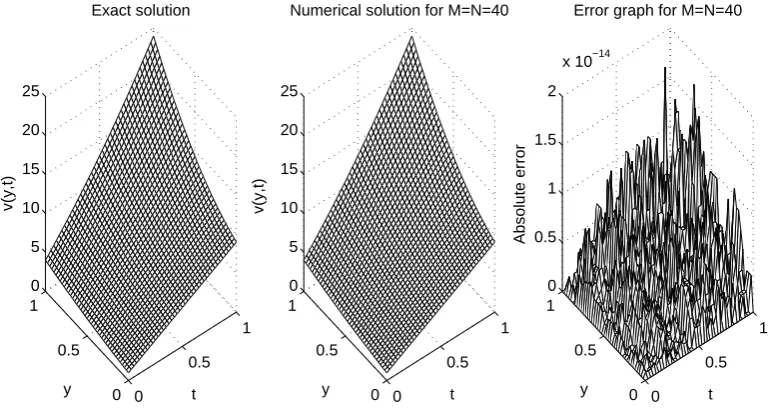
3 +8t(1+2t). The numerical and exact solutions forv(y, t) are shown in Figure 1 and very good agreement is obtained. Tables 1 and 2 give the numerical heat flux at y= 0 and the numerical integral in comparison with the exact values, i.e. µ3 and µ4. These have been calculated using the following O(h2) finite-difference approximations for derivative and trapezoidal rule for integration:

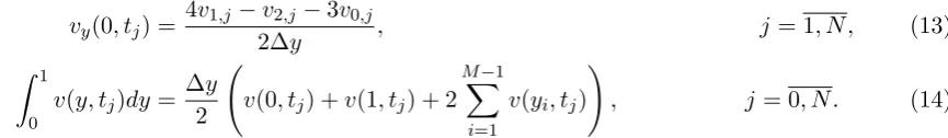
vy(0, tj) =

4v1,j−v2,j−3v0,j

2∆y , j= 1, N , (13)

∫ 1

0

v(y, tj)dy=

∆y

2 (

v(0, tj) +v(1, tj) + 2 M−1

∑

i=1

v(yi, tj)

)

, j= 0, N . (14)

From these tables it can be seen that the numerical results are in very good agreement with the exact ones and that a rapid monotonic decreasing convergence is achieved.

Table 1: The exact and the numerical heat flux−a(t)vy(0, t)/h(t) forM =N ∈ {10,20}, for the direct problem.

t 0.1 0.2 ... 0.8 0.9 1

M =N = 10 -2.2000 -2.4000 ... -3.6000 -3.8000 -4.0000

M =N = 20 -2.2000 -2.4000 ... -3.6000 -3.8000 -4.0000

exact -2.2000 -2.4000 ... -3.6000 -3.8000 -4.0000

Table 2: The exact and the numerical integralh(t)∫1

0 v(y, t)dy for M =N ∈ {10,20,40,100}, for the direct problem.

t 0.1 0.2 ... 0.8 0.9 1

M =N = 10 4.1789 6.5192 ... 31.8880 38.1539 45.0450

M =N = 20 4.1767 6.5158 ... 31.8660 38.1265 45.0113

M =N = 40 4.1762 6.5150 ... 31.8605 38.1196 45.0028

M =N = 100 4.1760 6.5147 ... 31.8590 38.1177 45.0005

0 0.5 1 0 0.5 1 0 5 10 15 20 25 t Exact solution y v(y,t) 0 0.5 1 0 0.5 1 0 5 10 15 20 25 t Numerical solution for M=N=40

y v(y,t) 0 0.5 1 0 0.5 1 0 0.5 1 1.5 2

x 10−14

t Error graph for M=N=40

y

Absolute error

Figure 1: Exact and numerical solutions forv(y, t) and the absolute error for the direct problem obtained withM =N= 40.

4

Numerical Approach for the Inverse Problem

In the inverse problem, we assume that the thermal diffusivity a(t) and free boundary h(t) are unknown. Usually, the nonlinear inverse problem (5)–(8) can be formulated as a nonlinear least-squares minimization. The regularized objective function which is minimized is given by

F(a, h) =

−a_h(₍t_t)₎vy(0, t)−µ3(t) 2 +

h(t)

∫ 1

0

v(y, t)dy₋µ4(t) 2

+β(

∥a(t)_∥2+_∥h(t)_∥2)

, (15)

where β _≥ 0 is a regularization parameter and the norm is usually the L2[0, T]-norm. The discretization of (15) is

F(a, h) =

N

∑

j=0 [

− aj

hj

vy(0, tj)−µ3(tj)

]2 + N ∑ j=0 [ hj ∫ 1 0

v(y, tj)dy−µ4(tj)

]2 +β   N ∑ j=0

a2_j+

N

∑

j=1

h2_j



. (16)

The unregularized case β = 0 yields the ordinary nonlinear least-squares method which is usually unstable. The minimization ofF subject to the physical constraintsa >0 andh >0 is accomplished using the MATLAB toolbox routinelsqnonlin, which does not require supplying (by the user) the gradient of the objective function, [9]. The routinelsqnonlin attempts to find a minimum of a scalar function of several variables, starting from an initial guess, subject to constraints and this generally is referred to as a constrained nonlinear optimization.

We take bounds for the positive quantities a(t) and h(t) say, we seek them in the interval (10−10_,103_{). We also take the parameters of the routine as follows:}

• Maximum number of iterations = 102_{×(number of variables).}

• Maximum number of objective function evaluations = 103_{×(number of variables).} • x Tolerance (xTol) = 10−10_.

• Function Tolerance (FunTol) = 10−10_. • Nonlinear constraint tolerance = 10−6_.

We take the initial guess as a(0) _=h(0) _{= 1. It is worth mentioning that at the first time step,} i.e. j= 0, the derivative vy(0,0) is obtained from (10) and (13), as

vy(0,0) =

4ϕ1−ϕ2−3ϕ0

2∆y , (17)

whereϕi =ϕ(h0yi) fori= 0, M. In addition, when we solve the inverse problem we approximate

h′ (tj) =

h(tj)−h(tj−1)

∆t =

hj−hj−1

∆t , j= 1, N . (18)

We also expressh′_{(0) as}

h′

(0) = µ ′

2(0)−a(0)ϕ′′(h0)−f(h0,0)

ϕ′_(h 0)

, (19)

which can easily be derived from equation (3) using the chain rule technique. In (19), a(0) is unknown.

If there is noise in the measured data (8), we replaceµ3(tj) andµ4(tj) in (16) byµϵ31(tj) and

µϵ2

4 (tj), namely,

µ₃ϵ1(tj) =µ3(tj) +ϵ1j, µ4ϵ2(tj) =µ4(tj) +ϵ2j, j= 0, N , (20)

where ϵ1j and ϵ2j are random variables generated from a Gaussian normal distribution with

mean zero and standard deviationsσ1 and σ2, respectively, given by

σ1 =p× max

t∈[0,T]|µ3(t)|, σ2=p×tmax∈[0,T]|µ4(t)|, (21) whereprepresents the percentage of noise. We use the MATLAB functionnormrnd to generate the random variablesϵ1 and ϵ2 as follows:

ϵ1 =normrnd(0, σ1, N + 1), ϵ2 =normrnd(0, σ2, N + 1). (22)

5

Numerical Results and Discussion

The numerical results are illustrated for two different examples according to the linear or non-linear variation of estimated coefficients. In addition, we add noise, as in (20), to the measured input data (8). To compute the thermal diffusivity a(t) and the free boundary h(t) we use the

lsqnonlin routine from MATLAB optimization toolbox with the Trust-Region-Reflective algo-rithm, [9], to find the minimizer of the nonlinear Tikhonov regularization functional (16). We have also calculated the root mean square error (rmse) to analyse the error between the exact and estimated solution, defined as,

rmse(a(t)) = v u u t

1

N + 1

N

∑

j=0

(anumerical(tj)−aexact(tj))2, (23)

rmse(h(t)) = v u u t

1

N

N

∑

j=1

(hnumerical(tj)−hexact(tj))2. (24)

Example 1

Consider the problem (1)–(4) with unknown coefficients a(t) and h(t), and solve this inverse problem with the following input data:

µ1(t) = 1 + 8t, µ2(t) = (2 + 2t)2+ 8t, µ3(t) =−2(1 +t),

µ4(t) =

(2 + 2t)3₋1

3 + 8t(1 + 2t), h0 = 1, ϕ(x) = (1 +x)

2_{, f(x, t) = 6} −2t.

One can remark that the conditions of Theorem 2 are satisfied hence, the uniqueness of solution holds. With this data the analytical solution is given by

a(t) = 1 +t, h(t) = 1 + 2t, u(x, t) = (1 +x)2+ 8t. (25)

Then

a(t) = 1 +t, h(t) = 1 + 2t, v(y, t) =u(yh(t), t) = (1 +y(1 + 2t))2+ 8t, (26)

is the analytical solution of the problem (5)–(8).

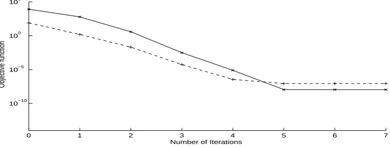
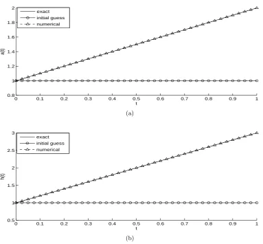
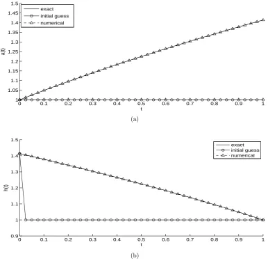
Consider first the case where there is no noise in the input data (8). The objective function (16), as a function of the number of iterations, is represented in Figure 2. From this figure it can be seen that the convergence is rapidly achieved in a few iterations. The objective function (16) decreases rapidly and takes a stationary value ofO(10−8_{) in about 7 iterations. The numerical} results for the corresponding unknownsa(t) andh(t) are presented in Figure 3. From this figure it can be seen that the retrieved thermal diffusivitya(t) and free surfaceh(t) are in very good agreement with the exact values from (26).

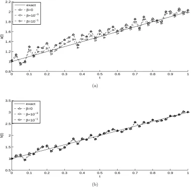
Next, we add p = 2% noise to the measured data µ3 and µ4, as in equation (20). The regularized objective function (16) is plotted, as a function of the number of iterations, in Figure 4 and convergence is again rapidly achieved. Figure 5 presents the graphs of the recovered functions, whilst the rmse values are given in Table 3. From this figure and table it can be seen that there is not much difference between the numerical solution obtained with β = 0 or

β= 10−3_{, but there is some slight improvement in accuracy obtained for β= 10}−1_.

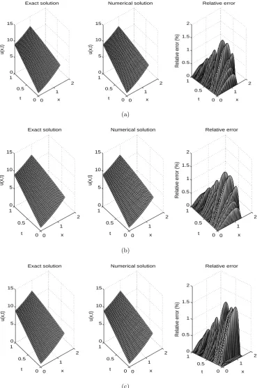
The recovered temperatures for β_{∈ {}0,10−3_,10−1_{}are shown in Figure 6. From this figure} it can be seen that the temperature component of the solution is stable and is not significantly affected by the inclusion of noise in the input data.

0 1 2 3 4 5 6 7

10−10 10−5 100 105

Number of Iterations

Objective function

0 0.1 0.2 0.3 0.4 0.5 0.6 0.7 0.8 0.9 1 0.8

1 1.2 1.4 1.6 1.8 2

t

a(t)

exact initial guess numerical

(a)

0 0.1 0.2 0.3 0.4 0.5 0.6 0.7 0.8 0.9 1

0.5 1 1.5 2 2.5 3

t

h(t)

exact initial guess numerical

(b)

Figure 3: (a) Thermal diffusivitya(t), and (b) Free surface h(t), for Example 1 with no noise and no regularization.

0 2 4 6 8 10 12 14 16

10−2 10−1 100 101 102 103 104

Number of Iterations

Regularized objective function

β=0

β=10−3

β=10−1

0 0.1 0.2 0.3 0.4 0.5 0.6 0.7 0.8 0.9 1 0.8

1 1.2 1.4 1.6 1.8 2 2.2

t

a(t)

exact

β=0

β=10−3

β=10−1

(a)

0 0.1 0.2 0.3 0.4 0.5 0.6 0.7 0.8 0.9 1

0.5 1 1.5 2 2.5 3 3.5

t

h(t)

exact

β=0

β=10−3

β=10−1

(b)

Figure 5: (a) Thermal diffusivitya(t), and (b) Free surfaceh(t), for Example 1 withp= 2% noise and regularization.

Example 2

In this example we consider the inverse problem (5)–(8) with the following input data:

µ1(t) = 1 + 8t, µ2(t) = (1 +√2−t)2+ 8t, µ3(t) =−2√1 +t,

µ4(t) = (1 + √

2₋t)3₋₁

3 + 8t

√

2₋t, h0= √

2, ϕ(x) = (1 +√2x)2, f(x, t) = 8₋2√1 +t.

One can remark that the conditions of Theorem 2 are satisfied hence, the uniqueness of solution holds. The solution to this inverse problem is given by

a(t) =√1 +t, h(t) =√2₋t, u(x, t) = (1 +x)2+ 8t. (27)

Then

0 2 4 0 0.5 1 0 5 10 15 20 25 x Exact solution t u(x,t) 0 2 4 0 0.5 1 0 5 10 15 20 25 x Numerical solution t u(x,t) 0 2 4 0 0.5 1 0 2 4 6 8 x Relative error t

Relative error (%)

(a) 0 2 4 0 0.5 1 0 5 10 15 20 25 x Exact solution t u(x,t) 0 2 4 0 0.5 1 0 5 10 15 20 25 x Numerical solution t u(x,t) 0 2 4 0 0.5 1 0 2 4 6 8 x Relative error t

Relative error (%)

(b) 0 2 4 0 0.5 1 0 5 10 15 20 25 x Exact solution t u(x,t) 0 2 4 0 0.5 1 0 5 10 15 20 25 x Numerical solution t u(x,t) 0 2 4 0 0.5 1 0 2 4 6 8 x Relative error t

Relative error (%)

(c)

Figure 6: (a) Temperature forβ = 0, (b)β= 10−3, and (c)β= 10−1, for Example 1 withp= 2% noise.

good agreement with the exact values from (28).

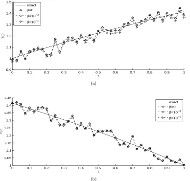
Next, we add p = 2% noise to the measured data µ3 and µ4, as in equation (20). The regularized objective function (16) is plotted, as a function of the number of iterations, in Figure 8 and convergence is again rapidly achieved. Figures 9 and 10 show the numerical solution (a(t), h(t), u(x, t)) and thermse values are given in Table 3. As in Example 1, one can observe that the inverse problem is rather stable with respect to noise included in the input data.

0 0.1 0.2 0.3 0.4 0.5 0.6 0.7 0.8 0.9 1

1 1.05 1.1 1.15 1.2 1.25 1.3 1.35 1.4 1.45 1.5

t

a(t)

exact initial guess numerical

(a)

0 0.1 0.2 0.3 0.4 0.5 0.6 0.7 0.8 0.9 1

0.9 1 1.1 1.2 1.3 1.4 1.5

t

h(t)

exact initial guess numerical

(b)

Figure 7: (a) Thermal diffusivitya(t), and (b) Free surface h(t), for Example 2 with no noise and no regularization.

Table 3: Thermsevalues for Examples 1 and 2 withp= 2% noise.

β = 0 β = 10−3 _{β= 10}−1

Example 1 rmse(a) = 0.1010 0.1004 0.0628

rmse(h) = 0.0932 0.0922 0.0872 Example 2 rrmse(a) = 0.0336 0.0336 0.0368

0 5 10 15 10−3

10−2 10−1 100 101 102

Number of Iterations

Regularized objective function

β=0

β=10−3

β=10−1

Figure 8: Regularized objective function (16), for Example 2 withp= 2% noise.

0 0.1 0.2 0.3 0.4 0.5 0.6 0.7 0.8 0.9 1

0.9 1 1.1 1.2 1.3 1.4 1.5

t

a(t)

exact

β=0

β=10−3

β=10−1

(a)

0 0.1 0.2 0.3 0.4 0.5 0.6 0.7 0.8 0.9 1

1 1.05 1.1 1.15 1.2 1.25 1.3 1.35 1.4 1.45

t

h(t)

exact

β=0

β=10−3

β=10−1

(b)

0 1 2 0 0.5 1 0 5 10 15 x Exact solution t u(x,t) 0 1 2 0 0.5 1 0 5 10 15 x Numerical solution t u(x,t) 0 1 2 0 0.5 1 0 0.5 1 1.5 2 x Relative error t

Relative error (%)

(a) 0 1 2 0 0.5 1 0 5 10 15 x Exact solution t u(x,t) 0 1 2 0 0.5 1 0 5 10 15 x Numerical solution t u(x,t) 0 1 2 0 0.5 1 0 0.5 1 1.5 2 x Relative error t

Relative error (%)

(b) 0 1 2 0 0.5 1 0 5 10 15 x Exact solution t u(x,t) 0 1 2 0 0.5 1 0 5 10 15 x Numerical solution t u(x,t) 0 1 2 0 0.5 1 0 0.5 1 1.5 2 x Relative error t

Relative error (%)

(c)

Figure 10: (a) Temperature for β = 0, (b)β = 10−3, and (c) β = 10−1, for Example 2 with p= 2% noise.

6

Conclusion

The resulting inverse problem has been reformulated as a nonlinear least-squares optimization problem which produced stable and reasonably accurate numerical results. Extension of the present work to include the determination of unknown convection b(t)ux and reaction c(t)u

coefficients in the heat equation (1), in addition to the unknownsa(t) andh(t), [10], will be the subject of future work.

Acknowledgments

M.S. Hussein would like to thank the Higher Committee of Education Development in Iraq (HCEDiraq) for their financial support in this research. The authors would also like to thank Professor M. Ivanchov for discussions on the subject of the paper.

References

[1] Cannon, J.R. (1984) The One-dimensional Heat Equation, Addison-Wesley, Menlo Park, California.

[2] Malyshev, I.G. (1975) Inverse problems for the heat-conduction equation in a domain with a moving boundary, Ukrainian Mathematical Journal,27, 568–572.

[3] Hon, Y.C. and Li, M. (2008) A computational method for inverse free boundary determina-tion problem,International Journal for Numerical Methods in Engineering,73, 1291–1309.

[4] Johansson, B.T., Lesnic, D. and Reeve, T. (2011) A method of fundamental solutions for the one-dimensional inverse Stefan problem, Applied Mathematical Modelling,35, 4367-4378.

[5] Shidfar, A. and Karamali, G.R. (2005) Numerical solution of inverse heat conduction prob-lem with nonstationary measurements, Applied Mathematics and Computation, 168, 540– 548.

[6] Lesnic, D., Elliott, L. and Ingham, D.B. (1998) The solution of an inverse heat conduction problem subject to the specification of energies, International Journal of Heat and Mass

Transfer,74, 25–32.

[7] Ivanchov, M.I. (2003) Inverse problem with free boundary for heat equation, Ukrainian

Mathematical Journal,55, 1086–1098.

[8] Smith, G.D. (1985)Numerical Solution of Partial Differential Equations: Finite Difference Methods, Oxford Applied Mathematics and Computing Science Series, Third edition.

[9] Mathwoks R2012 Documentation Optimization Toolbox-Least Squares (Model Fitting) Al-gorithms, available from www.mathworks.com/help/toolbox/optim/ug

/brnoybu.html.