Optimization of Adaptation - A Multi-objective Approach for Optimizing Changes to Design Parameters

This is a repository copy of

Optimization of Adaptation - A Multi-objective Approach for

Optimizing Changes to Design Parameters

.

White Rose Research Online URL for this paper:

http://eprints.whiterose.ac.uk/98439/

Version: Accepted Version

Proceedings Paper:

Salomon, S., Avigad, G., Fleming, P.J. orcid.org/0000-0001-9837-8404 et al. (1 more

author) (2013) Optimization of Adaptation - A Multi-objective Approach for Optimizing

Changes to Design Parameters. In: Evolutionary Multi-Criterion Optimization. 7th

International Conference, EMO 2013, March 19-22, 2013, Sheffield, UK. Lecture Notes in

Computer Science, 7811 . Springer Berlin Heidelberg , pp. 21-35. ISBN

978-3-642-37139-4

https://doi.org/10.1007/978-3-642-37140-0_6

[email protected] https://eprints.whiterose.ac.uk/

Reuse

Unless indicated otherwise, fulltext items are protected by copyright with all rights reserved. The copyright exception in section 29 of the Copyright, Designs and Patents Act 1988 allows the making of a single copy solely for the purpose of non-commercial research or private study within the limits of fair dealing. The publisher or other rights-holder may allow further reproduction and re-use of this version - refer to the White Rose Research Online record for this item. Where records identify the publisher as the copyright holder, users can verify any specific terms of use on the publisher’s website.

Takedown

If you consider content in White Rose Research Online to be in breach of UK law, please notify us by

Optimization of Adaptation - a Multi-Objective

Approach for Optimizing Changes to Design

Parameters

Shaul Salomon1_{, Gideon Avigad}2_{, Peter J. Fleming}1_{, and Robin C. Purshouse}1

1

Department of Automatic Control and Systems Engineering University of Sheffield

Mappin Street, Sheffield S1 3JD, UK

{s.salomon,p.fleming,r.purshouse}@sheffield.ac.uk

2 _{Department of Mechanical Engineering}

ORT Braude College of Engineering, Karmiel, Israel

[email protected]

Abstract. Dynamic optimization problems require constant tracking of the optimum. A solution for such a problem has to be adjustable in order to remain optimal as the optimum changes. The manner of changing de-sign parameters to predefined values is dealt with in the field of control. Common control approaches do not consider the optimality of the design, in terms of the objective function, while adjusting to the new solution. This study highlights the issue of the optimality of adaptation, and de-fines a new optimization problem – ”Optimization of Adaptation”. It is a multiobjective problem that considers the cost of the adaptation and the optimality while the adaptation takes place. An evolutionary algo-rithm is proposed in order to solve this problem, and it is demonstrated, first, with an academic example, and then with a real life application of a robotic arm control.

Keywords: dynamic optimization, adaptation, optimal control

1

Introduction

The necessity for adaptation may be also related to engineering (e.g., a prod-uct should be adapted to changes in market demands), companies (e.g., change of personnel or facilities, as costs change), politics, and many other fields of in-terest. In engineering design, adaptation may be ensured by including tunable parameters that can be altered when changes are required.

In the context ofsingle objective optimization, an initial design might lose its optimality as time passes due to changes that influence the objective function, or it might become infeasible with the changing of constraints. A tunable design may be able to adapt in order to maintain satisfactory performance, or to remain feasible, when such changes occur. This virtue avoids the need for producing a totally new design whenever an environmental change occurs, and it enables prolonging the lifetime of a product.

These kinds of optimization problems, where the optimal solution changes with time, are known as dynamic optimization problems (DOPs). Mathemati-cally, adynamic single objective optimization problem is formulated as follows:

Definition 1. Dynamic single objective optimization problem:

max x∈Qf(x, t)

s.t. gi(x, t)≥0, (i= 1, . . . , I)

hj(x, t) = 0, (j = 1, . . . , J)

whereQ⊂RM is the search domain,f is the objective function, andg and

h are the inequality and equality constraints, respectively. Since the objective function and the constraints are time dependent, the optimal solution ˜x also changes with time: ˜x⇒x˜(t).

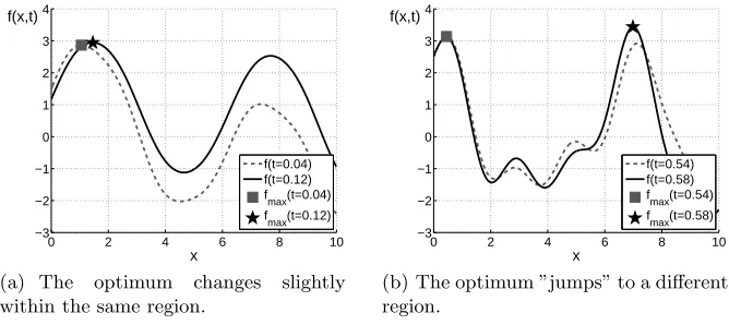
Many methods, including evolutionary algorithms, have been developed in order to solve DOPs, and to determine what changes should be performed in order to achieve optimal or satisfactory performance over time [5]. In many cases, the required changes in design over time are continuous and relatively small. In other cases, the optimum might ”jump” to a different region of the design space. This can happen when a totally different solution becomes the optimum, or when the current optimal solution becomes infeasible. The former case is illustrated in Figure 1. The dynamic functionf(x, t) = 2sin(x+ 2t) +tsin(3x−t) +cos(3xt) is presented at several time instants. In Figure 1(a) the optimal solution changes slightly between t = 0.04 and t = 0.12. On the other hand, in Figure 1(b), a new optimal solution is developed in the region of x= 7, and a ”jump” of the optimum occurs between the time instants t = 0.54 and t = 0.58. Since the required changes in design at times of an optimum ”jump” are significant, some issues regarding the manner of performing these changes should be considered.

0 2 4 6 8 10 −3

−2 −1 0 1 2 3 4

x f(x,t)

f(t=0.04) f(t=0.12) f

max(t=0.04)

f_max(t=0.12)

(a) The optimum changes slightly

within the same region.

0 2 4 6 8 10

−3 −2 −1 0 1 2 3 4

x f(x,t)

f(t=0.54) f(t=0.58) f

max(t=0.54)

f_max(t=0.58)

(b) The optimum ”jumps” to a different region.

Fig. 1.A dynamic function at four time instants. The optimum changes from the grey square to the black star.

the old and the new solutions), the function values during the adaptation are not optimal.

Although existing research has addressed finding efficient ways to track the moving optimum, no research known to the authors has addressed the optimality during the change itself. This study comes to shed some light on this issue. The aim here is not to suggest a new method for solving DOPs, but to optimize the adaptation of a solution when it requires significant changes. It is assumed here that the DOP is already solved, and the new location of the optimum is known. The aim is at designing a trajectory in phase plane (high level control design), according to its related performances in objective space. This is in contrast to the common approach in control theory, where the optimization is based on the trajectories in phase plane (e.g., minimizing the states’ deviation from the new set-point).

In many cases, changing a system’s design has a cost, in terms of money, energy or other resources. The way parameters are changed, especially when more than one parameter is to be adjusted, may affect the cost of the change. The possible conflict between the optimality of the performance during the change, and the cost of the adaptation defines a new optimization problem which is termed here as- Optimization of Adaptation. It is amulti-objective optimization problem (MOP) by its nature, since the function value during the adaptation process, and the cost of the change are to be optimized at the same time.

x₁ x₂

−6 −4 −2 0 2 4 6

−6 −4 −2 0 2 4

6 _f

x

0

x

f

Traj

1

Traj

2

Fig. 2.Two possible trajectories to adapt fromx0toxf. Brighter contour lines

repre-sent higher function values.

0 0.05 0.1

−1.5 −1 −0.5 0 0.5 1

t f

(a)

0 0.05 0.1

−1.5 −1 −0.5 0 0.5 1

t f

(b)

Fig. 3.The trajectoriesf(t) for the two trajectories of Figure 2. Figure 3(a) refers to trajectory 1, and Figure 3(b) refers to trajectory 2.

2

Methodology

2.1 Problem Definition

In order to optimize the adaptation of a system at a time instanttjump, when a significant change in design is required, the following assumptions are made:

1. The change takes place over a time interval [t0, tf] which is significantly shorter than the time constant of the DOP. Hence, the function value and the constraints can be considered as static for the duration of the change:

f(x, tjump) =f(x)

gi(x, tjump) =gi(x)

hj(x, tjump) =hj(x)

2. The state of the design parameters prior to the change is x(t0) =x0. 3. The state of the design parameters at the end of the change is the new

op-timal solution of the DOP: x(tf) = xf , f(xf) = maxf(x) (assuming maximization).

4. The system is at a steady state at the beginning and at the end of the adaptation.

Considering the above assumptions, the new optimization problem is defined as follows:

Definition 2. Optimal adaptation problem (OAP):

min

x(t)∈Q{Error(

x(t)), Cost(x(t))} , t∈[t0, tf] (1)

s.t. x(t0) =x0 , x(tf) =xf (2)

dx dt t0

= dx dt tf

= 0 (3)

gi(x(t))≥0 , (i= 1, . . . , I) (4)

hj(x(t)) = 0, (j= 1, . . . , J) (5)

where x(t) is a trajectory in the design space for the entire time interval,

Error(x(t)) is the difference between the function value at timetand the optimal function valuef(xf):Error(x(t)) =f(xf)−f(x(t)), andCost(x(t)) represents the invested resources for changing x from x0 to xf. The constraints of the original DOP (Eq. (4) and (5)) must be met at all times.

2.2 Assessment of the Objective Functions

Each solution for the proposed problem is a trajectory, and its resulting perfor-mances in the objective space (Error, Cost), as defined previously, are trajec-tories as well. Some research exists on the optimization of trajectrajec-tories (e.g. [6]), but the common approach is to represent each trajectory by an auxiliary func-tion (e.g. [7],[8]). In this paper we adopt this approach, and assess the objective functions by using a common concept from optimal control theory:

– The error functionError(x(t)) is represented by itsintegral absolute(IAE), which is a well known measure of optimality in control theory:

IAE=

tf

R

t0

|f(xf)−f(x(t))|dt

Recalling the trajectories in Figure 3, theIAEof each trajectory is equal to the area in between the function value and the optimal value marked with the dashed line. It is clear that theIAE of the trajectory in Figure 3(b) is smaller than theIAE of the trajectory in Figure 3(a).

– The cost functionCost(x(t)) is represented by the overall cost of the control forces required to follow the trajectory x(t). It is assumed here that the design variables are controlled by a vector of control forcesu= [u1, . . . , up]T, where each design variable is controlled by one or more control variables. Every control force has its cost, and the total costC is calculated as follows:

C=

tf

R

t0

wT_u(t) dt

wherewis a cost vector withwi represents the cost ofui. Each control force variableui has its related saturation values, which define the domain of the control forces.

The OAP may now be reformulated by changing the objectives at Eq. 1 in Definition 2, and by considering the saturation values as additional constraints. Because the objective functions are evaluated based on utility functions, the reformulated problem is presented here as:

Definition 3. Utility based Optimal Adaptation Problem (UOAP):

min

x₍t)∈Q{IAE, C} , t∈[t0, tf] (6)

s.t. x(t0) =x0 , x(tf) =xf (7)

dx dt t0

= dx dt tf

= 0 (8)

umin ≤u(t)≤umax (9)

gi(x(t))≥0 , (i= 1, . . . , I) (10)

wherex(t) =f(u(t)).

As is common in control,IAEandCare in conflict with one another. There-fore, the optimal solution for the UOAP, as is the case with the OAP, is expected to be a set rather than a single solution. Note that other reformulations for the OAP are possible.

3

Solving the Problem with an Evolutionary Algorithm

In this section, an evolutionary algorithm (EA) is presented for solving the UOAP, defined in Definition 3.

3.1 The Genotype

For a better visualisation of the problem, the value of the design variables are considered here as their positions. The first and second derivatives in time of the variables are considered as their velocityv(t) and accelerationa(t), respectively. Although the solution of the UOAP is the trajectoryx(t), it is coded bya(t).

The time interval is defined atKtime instants-t= [t1, . . . , tk, . . . , tK], where

t1=t0 andtK =tf. Each solution is defined by a matrix A of sizeM ×K of real coded variables.Amk represents the acceleration of themth design variable at thekth _{time sample.}

Considering the constraints in Eq. (7) and (8), the speedvm(t) and position

xm(t) can be derived as follows:

vm(t) = t Z

t0

am(t) dt (12)

xm(t) =x0m+ t Z

t0

vm(t) dt (13)

Of course, the integrals are evaluated by a discrete approximation method such as the trapezoidal rule, for example.

3.2 Constraint Satisfaction: Repair Method

In order to satisfy the constraints regardingtf in Eq. (7) and (8), two modifica-tions of the acceleration trajectory are made. The first results in an intermediate acceleration trajectorya(t)∗∗ _{which satisfies Eq. (8), and the second results in}

the repaired acceleration trajectorya(t) which satisfies Eq. (7) as well.

Let a pre-repair acceleration trajectory be a∗_{(t). It is clear from Eq. (12)}

that in order to force the final speed vm(tf) = 0, the mean acceleration has to be zero. This can be realized by subtracting from a∗_{(t) its mean value¯a}∗_.

intermediate velocity trajectoryv∗∗_{(t), using Eq. (12), satisfies the constraint of}

Eq. (8). Then the intermediate final position of the trajectoryx∗∗_(t

f) according to Eq. (13) is:

x∗∗

(tf) =x0+ tf Z

t0

v∗∗

(t) dt

At the second stage, in order to satisfy Eq. (7),a∗∗_{(t) is scaled by a scaling}

vectorl:

l= [l1, . . . , lm, . . . , lM] T

, lm=

xf m−x0m

x∗∗

m(tf)−x0m

The repaired final acceleration variable that satisfies both constraints is a(t) =a∗∗

(t)·l.

Although the suggested gene manipulation may result in violation of the constraint in Eq. (9), it speeds up the evolutionary process since it eliminates the two equality constraints in Eq. (7) and (8).

3.3 The Evolutionary Algorithm

All of the problems of Section 4 are solved using NSGA-II with constraint domi-nation [9]. The genetic operators used are the simulated binary crossover (SBX) operator and polynomial mutation [10], with distribution indexes ofηc= 15 and

ηm= 20 respectively. A cross-over probability ofpc= 1 and a mutation proba-bility ofpm = 1/M K are used. The stopping criterion is a maximal number of generations. A schema of the EA is presented in Algorithm 1.

Algorithm 1The evolutionary algorithm for solving the UOAP

1: R∗

1 ←generate a random set of solutions of size2N

2: R1←modifyR∗1 according to the procedure in Section 3.2

3: g←1

4: while_{g≤number of generations}do

5: evaluateRg

6: Pg+1←selectN solutions fromRg

7: Q∗

g+1←evolve fromPg+1(cross-over and mutation)

8: Qg+1←modifyQ∗g+1according to the procedure in Section 3.2

9: Rg+1←Pg+1∪Qg+1

10: g←g+ 1

4

Test Cases

4.1 Academic Example

Consider the following unconstrained DOP:

max

x f(x, t) =

sin (x1+x2+t/20) x22+ 1

−cos x1−x2+ (t/10000)

2_{+ 4}

x22+ 1

+x1 2

80

xi ∈[−2π,2π] , i={1,2}.

Whent= 98, the optimum ”jumps” fromx=x0= [3.24,−0.16]T tox=xf = [−3.24,−0.12]T_{. The contour of the function at t = 98, and the old and new} optima were previously depicted in Figure 2. The UOAP for the adaptation in that time instant is solved by the EA described in Algorithm 1. The adaptation’s time interval is set to 0.1, and it is defined for K = 30 time instants. The population consists of 250 members, and it is evolved over 300 generations.

For this example, the design variables are considered as simple mechani-cal components that react to the control force according to Newton’s 2nd _law:

um(t) =imam(t), whereimis a constant number representing the inertia of the

mth _{design variable. Herei}

1= 20 andi2= 10.

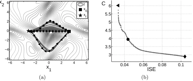
The set of non-dominated solutions in the final population is shown in Fig-ure 4. In FigFig-ure 4(a), the trajectories of all the non-dominated solutions are illustrated with gray lines. Three different trajectories from this set are marked with diamonds, triangles and circles. The trajectory marked with diamonds does not require investment of much control force, since it is aimed at the new op-timum with minimal changes possible. As a result, its cost is the lowest from all solutions. Since it runs through a region with very low function values, its

ISE is very high. The trajectory marked with circles passes along the highest function values on the way to the new optimum. As a result, it has a lowISE

value. In order to pass through these local optima, a significant force is required to be applied. Therefore, this solution has a highCvalue. The trajectory marked with diamonds is a compromise between the two objectives. Its path is shorter than the one of the circles, but it passes through only one local optimum. These insights can be depicted from the Pareto front shown in Figure 4(b). All of the non-dominated solutions are marked with gray dots, and the above three solutions are marked with black markers.

The control forces, positions and function values over time of these three solutions are shown in Figure 5. As mentioned in Section 2.2, the area under the control force function indicates the cost of the adaptation, and the area between the function value in time and the optimal function value indicates the ISE. The trade-off between optimality over time and the cost of the adaptation can be seen here. A larger area of the control force is associated with a smaller area of the error, and vice versa.

settings. For three of the 100 simulations the algorithm failed to find the tra-jectories with the lowestISE values, such as the triangle associated solution in Figure 4. The lowestISE value in these cases was 0.04.

x₁ x

2

−6 −4 −2 0 2 4 6 −6

−4 −2 0 2 4 6

f x

0

x

f

(a)

0.04 0.06 0.08 0.1 3

3.5 4 4.5 5 5.5 6

ISE C

(b)

Fig. 4.The final approximated set of the UOAP. Three different trajectories are marked in Figure 4(a), and their associated objective values are marked in Figure 4(b).

4.2 Real World Example

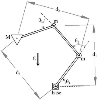
To demonstrate the scope of the proposed optimization approach, the following engineering problem is introduced. A planar robot with three rotating links of equal lengths has to carry a load of mass M over a specific route. The angles of the joints are controlled by the user with servo motors that are free to rotate at any angle. The mass of each motor is m. The robot and related parameters are depicted in Figure 6. The desired location of the load, i.e., the end of the robot’s third link, is progressing very slowly. Since it has three degrees of freedom, the robot can keep the load at the desired location with an infinite number of configurations. The optimization goal is to follow the path while minimizing the robot’s dimensions, i.e., keeping it as folded into itself as possible. Thisdynamic optimization problem can be formulated as follows:

min θ₍t)∈_R3φ(

θ_{(t)) (14)}

s.t. re=P(t) (15)

0 0.05 0.1 −1 0 1 t f

0 0.05 0.1 −2 0 2 t x 1

0 0.05 0.1 −5 0 5 t u 1

0 0.05 0.1 −4 −2 0 2 t x 2

0 0.05 0.1 −4 −2 0 2 4 t u 2

(a) First solution – a high error and low cost.

0 0.05 0.1 −1

0 1

t f

0 0.05 0.1 −2 0 2 t x 1

0 0.05 0.1 −5 0 5 t u 1

0 0.05 0.1 −4 −2 0 2 t x 2

0 0.05 0.1 −4 −2 0 2 4 t u 2

(b) Second solution – a low error and high cost.

0 0.05 0.1 −1

0 1

t f

0 0.05 0.1 −2 0 2 t x 1

0 0.05 0.1 −5 0 5 t u 1

0 0.05 0.1 −4 −2 0 2 t x 2

0 0.05 0.1 −4 −2 0 2 4 t u 2

(c) Third solution – a compromise between error and cost.

Fig. 5. The control forces, positions and function values over time for the solutions highlighted in Figure 4.

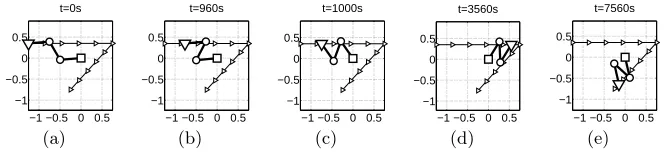
depicts the solution of the above DOP. The required path of the load P(t) is marked with arrows, and the optimal configuration is shown for five time in-stants. When the robot’s end is located far from the base, such as in Figures 7(a) and 7(b), the configuration with minimal dimensions has a ”Z” shape. When it is closer to the base, such as in Figures 7(c) and 7(d), the optimal configuration has an ”N” shape. For the example given, when t= 1000sthe robot has to change its configuration from ”Z” to ”N”. The duration of the change is 4 seconds. The question of how to perform that change is considered as the following utility optimal adaptation problem. The UOAP follows the main optimization goal, i.e. minimizing the dimensions of the robot, and it also seeks to minimize the power applied to the motors:

min

θ₍t)∈R3{E, C} , t∈[t0, tf]

s.t. θ_{(t0) =}θ0 , θ(tf) =θf dθ

dt t0

=dθ dt tf

= 0

−τ_sat≤τ_(t)≤τ_sat

where τ_{(t) = [τ1(t), τ2(t), τ3(t)]}T _{is a vector with the required torques in the}

joints to follow the trajectoryθ_(t),τ_{sat are the saturation values of the motors,}

E is the integral ofφ(t), andC is the total applied torque over time:

E=

tf

R

t0

φ(t) dt , C= tf

R

t0

_P3

i=1|τi(t)|

dt.

θ0 and θf are the configurations at Figure 7(b) and 7(c), respectively.u(t) is calculated by the iterative Newton-Euler dynamic formulation (for more infor-mation, see [11]).

−1 −0.5 0 0.5 −1

−0.5 0 0.5

t=0s

(a)

−1 −0.5 0 0.5 −1

−0.5 0 0.5

t=960s

(b)

−1 −0.5 0 0.5 −1

−0.5 0 0.5

t=1000s

(c)

−1 −0.5 0 0.5 −1

−0.5 0 0.5

t=3560s

(d)

−1 −0.5 0 0.5 −1

−0.5 0 0.5

t=7560s

(e)

Fig. 7.The configurations with minimal dimensions for five positions of the load. The manipulator’s base is marked with a square, and the load is marked with a triangle. The initial configuration of the OAP is the one at Figure 7(b), and the the final configuration is the one at Figure 7(c).

trajectories. Note that the above UOAP is different from the common approach arising from using optimal control theory for designing optimal controllers. A controller designed according to optimal control theory considers the final state

θf as an optimization goal, and tries to minimize the control force and the error fromθf. In contrast, here, the optimization goal is the original goal of the DOP, i.e., minimizing the dimensions of the robot.

3 3.05 3.1 3.15 60

65 70 75 80 85 90 95

Total Extent [m*s]

Total Torque [N*m*s]

Fig. 8.The approximated set of Pareto optimal solutions for the UOAP, found by the EA.

The UOAP was solved by the EA described in Algorithm 1, using the same configuration parameters as in the academic example from the previous section. The final approximated set is depicted in Figure 8. The two extreme solutions, marked with a larger circle and diamond, are shown in Figures 9 and 10. The trajectories of the torques, the joint angles and the extent are shown in Figure 9, and the dynamic behavior of the robot is shown in Figure 10. Note that in order to fold more quickly, under the limits of the saturation torque values, the solution marked with a circle rotates around its base. The solution marked with a diamond balances vertically until it needs to stretch again in the other configuration.

5

Conclusions and Future Work

0 2 4 0.5 1 1.5 t Φ

0 2 4

2 4 6 8 t θ₁

0 2 4

−40 −20 0 20 t M 1

0 2 4

2.5 3 3.5 4 t θ₂

0 2 4

−15 −10 −5 0 5 t M 2

0 2 4

2.5 3 3.5 4 t θ₃

0 2 4

−20 −10 0 10 t M 3

(a) One alternative – small dimensions and high cost. Note that the finalθ1is 2πlarger

than the desired final value. That means the manipulator performs a full turn around its base.

0 2 4

0.5 1 1.5

t Φ

0 2 4

2 4 6 8 t θ₁

0 2 4

−40 −20 0 20 t M 1

0 2 4

2.5 3 3.5 4 t θ₂

0 2 4

−15 −10 −5 0 5 t M 2

0 2 4

2.5 3 3.5 4 t θ₃

0 2 4

−20 −10 0 10 t M 3

(b) Second alternative – larger dimensions and smaller cost.

Fig. 9.Trajectories of the joint torques and angles and the extent of the robot in time.

−1 0 1

−1 0 1

t=0.4s

−1 0 1

−1 0 1

t=1s

−1 0 1

−1 0 1

t=2s

−1 0 1

−1 0 1

t=3s

−1 0 1

−1 0 1

t=4s

(a) One alternative – small dimensions and high cost.

−1 0 1

−1 0 1

t=0.4s

−1 0 1

−1 0 1

t=1s

−1 0 1

−1 0 1

t=2s

−1 0 1

−1 0 1

t=3s

−1 0 1

−1 0 1

t=4s

(b) Second alternative – larger dimensions and smaller cost.

EA was proposed in order to solve it. The EA was tested on two examples: a theoretic mathematical function and a problem of robotic arm control. For both examples, the EA was able to find a set of trade off solutions that enable the de-cision maker to choose whether to adapt in a minimum cost manner or to invest more resources in order to maintain high function values along the adaptation.

As future work, the new approach should be integrated and tested on more real life applications. This paper dealt with a single objective DOPs. The issue of optimal adaptation for multiobjective DOPs should be studied as well. The method should be also extended to deal with cases where the future function values and costs are subject to uncertainties.

Acknowledgements This research was supported by a Marie Curie Interna-tional Research Staff Exchange Scheme Fellowship within the 7th_European Com-munity Framework Programme.

References

1. Rose, M., Lauder, G.: Adaptation. Academic Press, San Diego, CA (1996) 2. Ferguson, G., Murphy, J., Ramanamanjato, J., Raselimanana, A., et al.: The

pan-ther chameleon: color variation, natural history, conservation, and captive man-agement. Krieger Publishing Company (2004)

3. Ruseckaite, R., Lamb, T., Pianta, M., Cameron, A.: Human scotopic dark adap-tation: Comparison of recoveries of psychophysical threshold and erg b-wave sen-sitivity. Journal of Vision11(8) (2011)

4. Jacobs, R., Lundby, C., Robach, P., Gassmann, M.: Red blood cell volume and the

capacity for exercise at moderate to high altitude. Sports Medicine 42(8) (2012)

643–663

5. Branke, J.: Evolutionary approaches to dynamic optimization problems-updated survey. In: GECCO Workshop on evolutionary algorithms for dynamic optimiza-tion problems. (2001) 27–30

6. Avigad, G., Eisenstadt, E., Goldvard, A., Salomon, S.: Transient responses opti-mization by means of set-based multi-objective evolution. Engineering Optimiza-tion44(4) (2011) 407–426

7. R´ene, M., J.J.S., Ole, S.: Topology optimization for transient response of photonic

crystal structures. Optical Society of America. Journal B: Optical Physics27(10)

(2010) 2040–2050

8. Toscano, R.: A simple robust pi/pid controller design via numerical optimization

approach. Journal of Process Control15(1) (2005) 81 – 88

9. Deb, K., Pratap, A., Agarwal, S., Meyarivan, T.: A fast and elitist multiobjective

genetic algorithm: Nsga-ii. Evolutionary Computation, IEEE Transactions on6(2)

(2002) 182–197

10. Deb, K., Agrawal, R.: Simulated binary crossover for continuous search space.

Complex systems9(2) (1995) 115–148