DOI:10.1051/0004-6361/201219657 c
ESO 2013
Astrophysics
&
The standard model of low-mass star formation applied to massive
stars: a multi-wavelength picture of AFGL 2591
,
K. G. Johnston
1, D. S. Shepherd
2, T. P. Robitaille
1, and K. Wood
31 Max Planck Institute for Astronomy, Königstuhl 17, 69117 Heidelberg, Germany e-mail:johnston@mpia.de
2 National Radio Astronomy Observatory, 1003 Lopezville Rd, Socorro, New Mexico 87801, USA 3 School of Physics & Astronomy, University of St Andrews, North Haugh, St Andrews, KY16 9SS, UK
Received 23 May 2012/Accepted 27 November 2012
ABSTRACT
Context.While it is currently unclear from a theoretical standpoint which forces and processes dominate the formation of high-mass stars, and hence determine the mode in which they form, much of the recent observational evidence suggests that massive stars are born in a similar manner to their low-mass counterparts.
Aims.This paper aims to investigate the hypothesis that the embedded luminous star AFGL 2591-VLA 3 (2.3 ×10⁵L
at 3.33 kpc)
is forming according to a scaled-up version of a low-mass star formation scenario.
Methods.We present multi-configuration Very Large Array (VLA) 3.6 cm and 7 mm, as well as Combined Array for Research in Millimeter Astronomy C18O and 3 mm continuum observations to investigate the morphology and kinematics of the ionized gas, dust, and molecular gas around AFGL 2591. We also compare our results to ancillary Gemini North near-IR images, and model the near-IR to sub-mm spectral energy distribution (SED) and Two Micron All Sky Survey (2MASS) image profiles of AFGL 2591 using a Monte-Carlo dust continuum radiative transfer code.
Results.The observed 3.6 cm images uncover for the first time that the central powering source AFGL 2591-VLA 3 has a compact core plus collimated jet morphology, extending 4000 AU eastward from the central source with an opening angle of<10◦at this radius. However, at 7 mm VLA 3 does not show a jet morphology, but instead compact (<500 AU) emission, some of which (<0.57 mJy of 2.9 mJy) is estimated to be from dust emission. The spectral index of AFGL 2591-VLA 3 between 3.6 cm and 7 mm was found to be between 0.4 and 0.5, similar to that of an ionized wind. If the 3.6 cm emission is modelled as an ionized jet, the jet has almost enough momentum to drive the larger-scale flow. However, assuming a shock efficiency of 10%, the momentum rate of the jet is not sufficient to ionize itself via only shocks, and thus a significant portion of the emission is instead likely created in a photoionized wind. The C18O emission uncovers dense entrained material in the outflow(s) from these young stars. The main features of the SED and 2MASS images of AFGL 2591-VLA 3 are also reproduced by our model dust geometry of a rotationally flattened envelope with and without a disk.
Conclusions.The above results are consistent with a picture of massive star formation similar to that seen for low-mass protostars. However, within its envelope, AFGL 2591-VLA 3 contains at least four other young stars, constituting a small cluster. Therefore it appears that AFGL 2591-VLA 3 may be able to source its accreting material from a shared gas reservoir while still exhibiting the phenomena expected during the formation of low-mass stars.
Key words.radiative transfer – techniques: interferometric – circumstellar matter – stars: formation – stars: massive – ISM: jets and outflows
1. Introduction
Does the formation of a massive star differ significantly from that of a low-mass star? Arguably, all studies of high mass (≥8M) star formation are centred upon this question. There are sev-eral possible reasons to expect differences at higher masses, one being that a massive star is thought to continue to accrete ma-terial after reaching the zero-age main sequence (ZAMS, e.g. Hosokawa et al. 2010), which is a consequence of its Kelvin-Helmholtz contraction time-scale being shorter than its accre-tion time-scale. Therefore, several processes such as radiaaccre-tion pressure (e.g.Yorke 2002) and ionization (e.g.Keto 2002) may
Figures 11 and 12 are available in electronic form at
http://www.aanda.org
FITS files are available at the CDS via anonymous ftp to
cdsarc.u-strasbg.fr(130.79.128.5) or via
http://cdsarc.u-strasbg.fr/viz-bin/qcat?J/A+A/551/A43
halt, decrease or alter accretion on to the star. However, in the earlier stages of protostellar evolution,Hosokawa et al.(2010) also find that the central accreting stars in their simulations be-come bloated due to accretion, so that the effective temperature and UV luminosity of the protostar remains low. Hence at ear-lier times these effects may be reduced. Secondly, while the den-sities and temperatures in pristine molecular clouds can easily explain the formation of low-mass star-forming cores, without the input of some stabilising energy such as an external pres-sure, micro-turbulence (McKee & Tan 2003), magnetic fields (e.g.Hennebelle et al. 2011;Commerçon et al. 2011) or radiative heating and outflows (e.g.Krumholz et al. 2012), these condi-tions are not conducive to creating a “monolithic” core that does not fragment, from which the forming massive star can accrete all of its mass. Instead, massive stars may start offembedded in smaller cores that source most of their mass from the surround-ing cluster-formsurround-ing clump (Bonnell et al. 2011;Myers 2011),
implying that massive stars can only form in clusters, not in isolation.
Placing these theoretical concerns aside initially, and work-ing under the hypothesis that massive stars form as a scaled-up version of low-mass star formation, in this paper we aim to probe the circumstellar environment of the massive star-forming re-gion AFGL 2591 by combining multi-wavelength observations and modelling to determine whether any of the signatures of its formation differ significantly from those of low-mass protostars. AFGL 2591 is a well-studied example of a luminous star-forming region (2.1−2.5×10⁵Lat 3.33 kpc,Lada et al. 1984; Henning et al. 1990;Rygl et al. 2012). One of its most promi-nent features is a one sided conical reflection nebula observed in the near-IR (e.gMinchin et al. 1991;Tamura & Yamashita 1992). Projected within the Cygnus-X star-forming complex, the distance to the source has recently been determined by trigono-metric parallax measurements to be 3.33±0.11 kpc, more dis-tant than previously assumed (between 1 and 2 kpc, e.g.Poetzel et al. 1992;Hasegawa & Mitchell 1995; Trinidad et al. 2003; van der Tak & Menten 2005). As will be described below, AFGL 2591 actually consists of several objects. However, as one source, AFGL 2591-VLA 3, dominates the spectral energy dis-tribution (SED) and infrared images and hence the luminosity, the name AFGL 2591 will therefore also be used henceforth to refer to this dominant source.
AFGL 2591 has been studied and modelled by many authors. For example, one-dimensional modelling of the circumstellar geometry via the observed SED has been carried out byGuertler et al.(1991);van der Tak et al.(1999);Mueller et al.(2002b) andde Wit et al. (2009). Improving on these,Preibisch et al. (2003) used two models – one of a disk and the other of an en-velope with outflow cavities – to reproduce the 40 AU diameter (assumingd =1 kpc) bright disk of emission observed in their K band image, andTrinidad et al.(2003) have modelled the mil-limetre emission from AFGL 2591-VLA 3 as an optically thick disk without an envelope. As part of their comprehensive study, van der Tak et al.(1999) modelled their observed molecular lines (CS, HCN, HCO+) including an outflow cavity in a power-law envelope, finding that a half-opening angle of 30◦ was able to better reproduce the line profiles.van der Wiel et al.(2011) have modelled a set of six lines detected toward AFGL 2591 as part of the JCMT Spectral Legacy Survey, finding evidence of a cav-ity or inhomogenecav-ity in the envelope on scales of≤ 104AU. In addition, as well as observing a bi-conical outflow struc-ture in12CO (2–1) on scales of 1−2 or several thousand AU, Jiménez-Serra et al.(2012) also uncovered evidence for chem-ical segregation within the inner 3000 AU of the AFGL 2591-VLA 3 envelope (assumingd = 3 kpc, similar to our assumed distance of 3.33 kpc).
The ionized gas emission in the region surrounding AFGL 2591 has previously been observed byCampbell(1984b); Tofani et al.(1995);Trinidad et al.(2003) and van der Tak & Menten(2005) from 5 to 43 GHz. These observations showed that AFGL 2591 is in fact not an isolated forming star, uncover-ing four continuum sources in the region. The observed fluxes of two of these, VLA 1 and VLA 2, gave spectral indices consistent with optically thin free-free emission from H
ii
regions, and a third source VLA 3, was measured to have a steeper spectral in-dex, possibly indicating optically thick emission. VLA 3 is also coincident with the central illuminating source of AFGL 2591 observed at shorter wavelengths (Trinidad et al. 2003). A fourth radio continuum source has also been detected by Campbell (1984a) andTofani et al.(1995) (their source 4 and n4 respec-tively), which shall be referred to as VLA 4 in the followingsections. In addition, the 3.6 cm images presented in this work uncover a fifth source, VLA 5, to the south west.
Knots of H2 and [SII] Herbig Haro objects have been de-tected toward AFGL 2591 (Tamura & Yamashita 1992;Poetzel et al. 1992), suggesting the presence of shocked gas. These are coincident with an east-west bipolar outflow (e.g. Lada et al. 1984;Hasegawa & Mitchell 1995), which extends across 5or 4.8 pc at 3.33 kpc, but also contains a more collimated central small-scale component with an extent of 90×20.
Evidence for the presence of a disk or rotationally flattened material around the central source of AFGL 2591 has been found by several authors. The near-IR imaging polarimetry observa-tions of Minchin et al. (1991) showed that a disk or toroid of material was needed to appropriately scatter the emission. In addition, a large (50× 80 ) flattened “disk” of mate-rial has been observed perpendicular to the outflow in obser-vations of CS lines (Yamashita et al. 1987). At smaller scales, van der Tak et al.(2006) andWang et al.(2012) found evidence for a disk of diameter 800 AU at 1 kpc (corresponding to 2700 AU at 3.33 kpc), which exhibits a systematic velocity gra-dient in the northeast-southwest direction. This gragra-dient was also found in the SMA observations ofJiménez-Serra et al.(2012), which they found to be consistent with Keplerian-like rota-tion around a 40 Mstar. Finally, both OH and water masers have been observed towards VLA 3 (Trinidad et al. 2003; Hutawarakorn & Cohen 2005; Sanna et al. 2012). The Very Large Array (VLA)1 22 GHz water maser observations of Trinidad et al.(2003) uncovered a maser cluster, which included a∼0.01diameter shell-like structure on the smallest scales. As well as finding largely consistent results, the Very Long Baseline Array 22 GHz water maser observations ofSanna et al.(2012) determined that the maser cluster is arranged in a v-shape, which coincides with the expected location of the outflow walls appar-ent in the near-IR reflection nebula.
In this paper, we have adopted a multi-wavelength approach to further probe the circumstellar environment of AFGL 2591, and to address the question of whether it forms in a similar man-ner to its low-mass counterparts. Building on previous work, the modelling presented in this paper includes the first simul-taneous radiative transfer model of the near-IR through sub-mm SED, and near-IR images, of AFGL 2591 with a three-dimensional axisymmetric geometry. In addition, we present new multi-configuration VLA 3.6 cm and 7 mm continuum ob-servations that for the first time trace an ionized jet at 3.6 cm, as well as13CO(1−0), C18O(1−0) and 3 mm continuum Combined Array for Research in Millimeter-wave Astronomy (CARMA2) observations, which trace previously unstudied scales within the molecular outflow and envelope, to derive a self-consistent picture of AFGL 2591.
Section2 outlines the new observations carried out in this work, describing both the VLA 3.6 cm and 7 mm, as well as the CARMA13CO, C18O and 3 mm continuum observations. Section3presents the archival data used in this paper, includ-ing near-IR to sub-mm SED, 2MASS photometry, measured 2MASS brightness profiles and Gemini North near-IR images of 1 Now the Jansky Very Large Array.
Table 1.Summary of VLA observations.
Wavelength Configuration Date of Program No. of Time Pointing centre Phase calibrator
observation antennas on-source (h) RA Decl. flux density (Jy)
3.6 cm A 2007 Jul. 26 AJ337 26 (22) 1.75 20 29 24.90 +40 11 21.00 (J2000) 1.49
3.6 cm B 2008 Jan. 18 AJ337 26 (21) 1.96 20 29 24.90 +40 11 21.00 (J2000) 1.91
3.6 cm C 2008 Mar. 9 AJ337 27 (23) 1.97 20 29 24.90 +40 11 21.00 (J2000) 2.13
3.6 cm D 2007 Apr. 12 AJ332 26 (20) 0.37 20 29 24.90 +40 11 21.00 (J2000) 1.25
7 mm A 2002 Mar. 25 AT273 27 (23) 1.97 20 27 35.95 +40 01 14.90 (B1950) 3.44
7 mm B 2008 Jan. 18 AJ337 26 (24) 3.43 20 29 24.90 +40 11 21.00 (J2000) 3.15
7 mm C 2008 Mar. 9 AJ337 27 (25) 4.18 20 29 24.90 +40 11 21.00 (J2000) 4.46
7 mm D 2007 Apr. 28 AJ332 26 (17) 0.44 20 29 24.90 +40 11 21.00 (J2000) 1.64
AFGL 2591. Section4describes the modelling of the near-IR to sub-mm SED and near-IR images. Section5presents the results for the SED and near-IR image modelling, as well as for the cen-timetre and millimetre wavelength datasets. Section6 presents our discussion, which covers the topics of the jet and outflow of VLA 3, and the properties of AFGL 2591 as a cluster. Our con-clusions are given in Sect.7.
2. Radio interferometric observations
2.1. VLA 3.6 cm and 7 mm continuum
Multi-configuration radio continuum observations at 3.6 cm and 7 mm were conducted between April 2007 and March 2008 with the VLA of the National Radio Astronomy Observatory3.
During this time frame, the VLA continuum mode consisted of four 50 MHz bands, two of which were placed at 8.435 GHz, and two at 8.485 GHz for 3.6 cm, and similarly two at 43.315 GHz and two at 43.365 GHz for 7 mm. At 3.6 cm, observations were taken in all four configurations of the VLA (A to D), and at 7 mm, observations were performed in B through D array and combined with A array archive data previously published in van der Tak & Menten(2005). When combined, these observa-tions provided baseline lengths between 35 m and 36.4 km, giv-ing information on angular scales from 0.24to 3for 3.6 cm, and 0.05 to 43for 7 mm.
For each observation, Table1lists the observed wavelength, configuration, observation date, program code, number of an-tennas in the array (with the number of anan-tennas with useful data shown in brackets), time on-source, the pointing centre of the target, and the flux density of the gain calibrator determined from bootstrapping the flux from the primary flux calibrator. The number of antennas with useful data was reduced due to anten-nas being out of the array for upgrading and testing of new VLA capabilities, general hardware issues, and also some residual bad data. For all observations, the gain calibrator was 2015+371 and primary flux calibrator was 1331+305 (3C286).
Data reduction and imaging were carried out using the Common Astronomy Software Applications (CASA)4package. As 1331+305 was slightly resolved, a model was used for flux calibration, which has a flux of 5.23 Jy at 3.6 cm and 1.45 Jy at 7 mm, allowing data at alluvdistances to be used. Antenna gain curves and an opacity correction (zenith opacity=0.06) were applied for the 7 mm data. The error in absolute flux calibration is approximately 1−2% for the 3.6 cm band, and 3−5% for the 7 mm band. The data were imaged using a CLEAN multi-scale deconvolution routine, using three scales, and Briggs weight-ing with a robust parameter of 0.5. The rms noise in the final 3 The National Radio Astronomy Observatory is a facility of the National Science Foundation operated under cooperative agreement by Associated Universities, Inc.
4 http://casa.nrao.edu
Table 2.Summary of radio interferometric observations.
λ Array line/ Synthesised beam Map rms
cont. size () PA (◦) (mJy beam−1)
3.6 cm VLA-A to D cont. 0.43×0.40 43 0.030
7 mm VLA-A to D cont. 0.11×0.11 43 0.056
3 mm CARMA-D 13CO 4.4×3.7 96 100
3 mm CARMA-D C18O 4.5×3.6 93 100
2.8 mm CARMA-D cont. 4.9×4.1 –4.8 2.2
2.7 mm CARMA-D cont. 4.3×3.5 95 2.1
combined images were 30 and 56μJy beam−1 for the 3.6 cm and 7 mm images respectively, and the synthesised beams were 0.43by 0.40, PA=43◦and 0.11by 0.11, PA=43◦. These values, as well as the synthesised beam and map rms for each part of the CARMA observations described in Sect.2.2, are sum-marised in Table2.
2.2. CARMA13CO, C18O and 3 mm continuum
CARMA observations atλ∼3 mm were taken on 10 July 2007 in D configuration (corresponding to baseline lengths between 11−150 m). A total of 14 antennas were used during the obser-vations, five 10-m and nine 6-m in diameter.
The CARMA correlator was comprised of two side bands, placed either side of the chosen LO frequency, which for these observations was 108.607 GHz. Both the upper and lower side bands contained three spectral windows: one wide and two nar-row, giving a total of six windows. The two wide spectral win-dows, centred on 106.7 and 110.5 GHz, had a bandwidth of 500 MHz and a total of 15 channels, and the four narrow spec-tral windows had a width of approximately 8 MHz and 63 chan-nels, giving a spectral resolution of 122 kHz. The observed lines, 13CO(J = 1−0) and C18O(J = 1−0), lay in the two nar-row spectral windows in the upper side band at 110.201 and 109.782 GHz. At these frequencies, the spectral resolution was
∼0.33 km s−1.
[image:3.595.309.553.230.311.2]Fig. 1.SED of AFGL 2591, collated from the literature. The best-fitting models for an envelope with and without a disk (overplotted solid blue and dashed red lines respectively) are discussed in Sect.5.1. The er-rors shown are those reset to 10% if the error in the measured flux was<10%.
results. To image the data, Briggs weighting and a robust param-eter of 0.5 were used. The beam size and rms noise for each ob-served line and continuum spectral window are given in Table2.
3. Archival data
3.1. SED
The observed near-IR to sub-millimetre SED of AFGL 2591 is shown in Fig.1. The SED data points were collected from the literature; Table3lists the wavelengths, flux densities and refer-ences for the data displayed in Fig.1. The 30 data points shown between 3.5 and 45μm were sampled uniformly in log-space from a highly processed ISO-SWS spectra of AFGL 2591 (Sloan et al. 2003) taken on 7 Nov. 1996, observation ID 35700734. The uncertainties for the averaged ISO-SWS spectrum were assumed to range from 4 to 22% as per the ISO handbook volume V5.
As mentioned in Sect.1, the SED and therefore flux densities of AFGL 2591 given in Table3were assumed to be dominated by one source. Evidence to support this assumption will be pre-sented in Sect.5.2.2, via a comparison of the SEDs of the re-solved sources in the region.
3.2. Near-IR 2MASS images
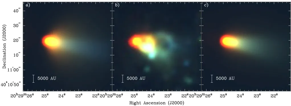
A three-colour 2MASS (Skrutskie et al. 2006)J,H, andKsband image of the near-IR emission observed towards AFGL 2591 is shown in the middle panel of Fig. 2, where red, green and blue areKs,HandJbands respectively. This Figure shows the conical near-IR reflection nebula (previously observed by e.g. Kleinmann & Lebofsky 1975;Minchin et al. 1991;Tamura & Yamashita 1992), which is consistent with being a blue-shifted outflow lobe from the central source of AFGL 2591.
To obtain integratedJ,HandKsband fluxes for AFGL 2591, irregular aperture photometry was performed on 2MASS Atlas images. Photometric uncertainties on the fluxes are<1%, how-ever it is likely the fluxes are more uncertain due to the choice of the irregular photometry apertures, and foreground or back-ground stars being included within them. The uncertainty due to 5 http://iso.esac.esa.int/users/handbook/
contaminating stars is likely dominated by the 2MASS source 20292393+4011105 at 20h29m23s.93 +40◦1110.56 (J2000; easily visible as a point source in the Gemini North near-IR im-ages presented in Sect.5.2), as the apertures were placed to avoid all other point sources visible in the 2MASS images. The fluxes of this contaminating source are 0.011, 0.035 and 0.105 Jy atJ,
HandKsbands respectively, withKsband being an upper limit. Therefore, the uncertainty in the measured 2MASS fluxes of the AFGL 2591 outflow lobe was estimated to be∼10%.
3.3. 2MASS brightness profiles
Flux profiles of AFGL 2591, summed across strips aligned with and perpendicular to the source outflow axis (PA=256◦, taken fromSanna et al.(2012), with thicknesses of 24.6 and 104 respectively), were measured for the three 2MASS bands. The background subtracted, normalised profiles are shown in Fig.3 along with the best-fitting models to both the SED and profiles, for the models consisting of an envelope with and without a disk (blue solid and red dashed lines respectively), which will be dis-cussed further in Sect.5.1. The background was determined by finding the average value within two strips either side of the main profile. The errors in the profiles shown in each panel of Fig.3 reflect the uncertainty due to background fluctuations, and are calculated as the standard deviation of the profiles measured in the two background strips, which were assumed to contain mini-mal source flux. As the strips used to calculate the uncertainty in the perpendicular profiles contained several bright stars, iterative sigma clipping was performed, i.e. pixels lying more than 5 stan-dard deviations away from the mean were then ignored and the mean and standard deviation were recalculated and the process was repeated until no pixels were rejected.
3.4. Near-IR gemini north NIRI images
High resolution near-IR images of AFGL 2591 were ob-tained from the Gemini website, which were taken under pro-gram GN-2001A-SV-20 as part of the commissioning of Gemini North’s NIRI instrument, and were available under public re-lease6. The total integration time was 2 min for J band and
1 min atHandKbands. We aligned the images using Chandra X-ray sources in the field (Evans et al. 2010), giving a positional accuracy of 0.6, and calibrated the flux level of the images in MJy sr−1using aperture photometry of bright sources in both the Gemini North and 2MASS images. The FWHMs of the PSFs in the images range between 0.3−0.4. The peak position of the central source of AFGL 2591 in theJband image was found to be 20h29m24s.86+40◦1119.5 (J2000), which was taken to be the position of the powering object. As these images were satu-rated inKband, 2MASS images were instead used for the mod-elling described in Sect.4. However, in Sects.5.2and5.3these high-resolution images are compared to the radio continuum and molecular line data observed for this work.
4. SED and near-IR image modelling
4.1. The dust continuum radiative transfer code
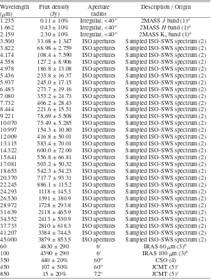
Table 3.Observed near-IR to sub-millimetre fluxes for AFGL 2591, collated from the literature.
Wavelength Flux density Aperture Description/Origin
(μm) (Jy) radius
1.235 0.11±10% Irregular,<40 2MASSJband (1)a
1.662 0.43±10% Irregular,<40 2MASSHband (1)a
2.159 2.30±10% Irregular,<40 2MASS Ksband (1)a 3.500 33.68±1.347 ISO apertures Sampled ISO-SWS spectrum (2) 3.822 68.98±2.759 ISO apertures Sampled ISO-SWS spectrum (2) 4.174 108.4±7.590 ISO apertures Sampled ISO-SWS spectrum (2) 4.558 127.2±8.906 ISO apertures Sampled ISO-SWS spectrum (2) 4.978 186.8±13.08 ISO apertures Sampled ISO-SWS spectrum (2) 5.436 233.8±16.37 ISO apertures Sampled ISO-SWS spectrum (2) 5.937 245.0±17.15 ISO apertures Sampled ISO-SWS spectrum (2) 6.483 273.7±19.16 ISO apertures Sampled ISO-SWS spectrum (2) 7.080 353.2±24.73 ISO apertures Sampled ISO-SWS spectrum (2) 7.732 406.2±28.43 ISO apertures Sampled ISO-SWS spectrum (2) 8.444 221.6±15.51 ISO apertures Sampled ISO-SWS spectrum (2) 9.221 78.69±5.508 ISO apertures Sampled ISO-SWS spectrum (2) 10.070 75.49±5.285 ISO apertures Sampled ISO-SWS spectrum (2) 10.997 154.3±10.80 ISO apertures Sampled ISO-SWS spectrum (2) 12.009 416.8±50.01 ISO apertures Sampled ISO-SWS spectrum (2) 13.115 583.4±70.01 ISO apertures Sampled ISO-SWS spectrum (2) 14.322 600.0±72.00 ISO apertures Sampled ISO-SWS spectrum (2) 15.641 556.8±66.81 ISO apertures Sampled ISO-SWS spectrum (2) 17.081 503.2±50.32 ISO apertures Sampled ISO-SWS spectrum (2) 18.653 542.3±54.23 ISO apertures Sampled ISO-SWS spectrum (2) 20.370 717.7±93.31 ISO apertures Sampled ISO-SWS spectrum (2) 22.245 886.1±115.2 ISO apertures Sampled ISO-SWS spectrum (2) 24.293 1118±145.3 ISO apertures Sampled ISO-SWS spectrum (2) 26.530 1391±180.9 ISO apertures Sampled ISO-SWS spectrum (2) 28.972 1728±293.8 ISO apertures Sampled ISO-SWS spectrum (2) 31.639 2118±465.9 ISO apertures Sampled ISO-SWS spectrum (2) 34.552 2413±530.9 ISO apertures Sampled ISO-SWS spectrum (2) 37.733 2810±618.3 ISO apertures Sampled ISO-SWS spectrum (2) 41.207 3384±744.5 ISO apertures Sampled ISO-SWS spectrum (2) 45.000 3879±853.5 ISO apertures Sampled ISO-SWS spectrum (2)
60 4830±290 6 IRAS 60μm (3)b
100 4390±290 6 IRAS 100μm (3)b
350 440±20% 60 CSO (4)
450 107±50% 60 JCMT (5)c
850 15±20% 72 JCMT (5)c
Notes.(a)Image shown in Fig.2. Fluxes found by irregular aperture photometry.(b)Fluxes found using radial aperture photometry on IRIS coadded images.(c)Fluxes found using radial aperture photometry on SCUBA Legacy Catalogue images.
References.(given in parentheses in the column Description/Origin): (1)Skrutskie et al.(2006); (2)Sloan et al.(2003); (3)Miville-Deschênes & Lagache(2005); (4)Mueller et al.(2002a); (5)Di Francesco et al.(2008).
genetic search algorithm used to model IRAS 20126+4104 in Johnston et al.(2011).
For a given source and surrounding dust geometry sampled in a spherical-polar grid, H
yperion
models the nonisotropic scattering and thermal emission by/from dust, calculating radia-tive equilibrium dust temperatures (using the technique ofLucy 1999), and producing spectra and multi-wavelength images. As dust and gas are assumed to be coupled in the code we are able to probe the bulk of the material which surrounds AFGL 2591. In this section, we describe the density structure of the disk, envelope and outflow cavity in the model.We model the circumstellar geometry of AFGL 2591 with the same 3D axisymmetric envelope with disk geometry suc-cessfully employed to model the SEDs and scattered light im-ages of low-mass protostars (e.g.Robitaille et al. 2007;Wood et al. 2002; Whitney et al. 2003). The axisymmetric three
dimensional flared disk density is described between inner and outer radiiRminandRdiskby
ρdisk(,z)=ρ0 R
0
α
exp⎧⎪⎪⎨⎪⎪⎩−1 2
z h()
2⎫⎪⎪ ⎬
⎪⎪⎭, (1)
whereR0 =100 AU,is the cylindrical radius,zis the height above the disk midplane andρ0 is set by the total disk mass
Fig. 2. a)Model three-colourJ,HandKsband image for the envelope with disk model (RGB:K,H, andJbands respectively).b)Observed 2MASS three-colour image of AFGL 2591.c)ModelJ,H, andKsband image for the envelope without disk model. The model images have been normalised to the total integrated fluxes given in Table3, in order that the morphology of the emission can be easily compared. Stretch: red:Ks band, 130−300 MJy sr−1; green:Hband, 95−150 MJy sr−1, blue:Jband, 30−60 MJy sr−1.
Eq. (1) is expressed in terms of R0 instead of R so that the scaleheight is defined at a radius which is more conceptually accessible.
The density of the circumstellar envelope is taken to be that of a rotationally flattened collapsing spherical cloud (Ulrich 1976;Terebey et al. 1984) with radiusRmax
env, ρenv(r, μ)=ρenv0
r Rc
−3/2 1+μμ
0 −1/2⎛
⎜⎜⎜⎜⎝μ μ0 +
2μ2 0Rc
r ⎞ ⎟⎟⎟⎟⎠−1
(2)
whereρenv0is the density scaling of the envelope,ris the spher-ical radius,Rc is the centrifugal radius,μ is the cosine of the polar angle (μ=cosθ), andμ0is the cosine of the polar angle of a streamline of infalling particles in the envelope asr→ ∞. The equation for the streamline is given by
μ3
0+μ0(r/Rc−1)−μ(r/Rc)=0 (3) which can be solved for μ0. In our model, we assume the centrifugal radius is also the radius at which the disk forms
Rc = Rdisk.
We chose to describe the envelope density via a density scal-ing factor instead of the envelope accretion rate and stellar mass used inJohnston et al.(2011), as this does not require the as-sumption of evolutionary tracks – which are currently very un-certain for massive stars – to provide a physical stellar radius and temperature for a given stellar mass. Instead, we have var-ied the stellar radius and temperature as parameters (described in Sect.4.2).
To reproduce the morphology of the emission in the near-IR images, we also include a bipolar cavity in the model geometry with densityρcav, and a shape described by
z()=z0bcav (4)
where the shape of the cavity is determined by the parameterbcav which we set to bebcav=1.5, andz0is chosen so that the cavity half-opening angle atz=10 000 AU isθcav. The cavity was in-cluded by resetting the envelope density toρcavinside the region defined by Eq. (4) only where the envelope density was initially larger.
The inner radius of the dust disk and envelopeRmin is ex-pressed in terms of the dust destruction radiusRsub, which was found empirically byWhitney et al.(2004) to be
Rsub=R(Tsub/T)−2.1 (5) where the temperature at which dust sublimates is assumed to be
Tsub=1600 K, andTis the temperature of the star. We adopted the dust opacity and scattering properties fromKim et al.(1994) for the circumstellar dust. This dust model has a ratio of total-to-selective extinctionRV =3.6 and a grain size distribution with
an average particle size slightly larger than the diffuse interstellar medium.
For the genetic algorithm, which is described in detail in Sect. 4.3 ofJohnston et al.(2011), the size of the first genera-tionN was set to 1000, and the size of subsequent generations
Mwas set to be 200. The code was taken to be converged when theχ2 value of the best fitting model decreased less than 5% in 20 generations.
4.2. Input assumptions: model parameters
A set of plausible ranges for parameters describing the model, in which the genetic algorithm searched for the best fit, is given in Table4. In addition to this, the stellar radius and tempera-ture were also required to lie above the zero-age main sequence defined as logTZAMS vs. log (0.9 ×RZAMS) for the solar metal-licity models ofSchaller et al.(1992), where the factor of 0.9 is to ensure that enough models are sampled around the ZAMS, rather than strictly above the ZAMS. The stellar temperatureT
and a stellar surface gravity of logg=4 were then used to select a model from the stellar atmosphere grid ofCastelli & Kurucz (2004). To sample the cavity half-opening angleθcav, we first determined the relation between the half-opening angle and the inclination such that the equation of the cavity, Eq. (4), projected onto the plane of the sky produced the right opening angle ob-served in the Gemini near-IR images,
i=arcsin
0.826 (sinθcav)b cosθcav ·
Fig. 3.Black error bars: normalised flux profiles for the three 2MASS bands, aligned with (top) and perpendicular to (bottom) the outflow axis. Blue and red lines: the profiles of the best-fitting models to both the observed SED and profiles, for envelope with disk and without disk models respectively. Vertical grey dashed lines mark the position of the central source.
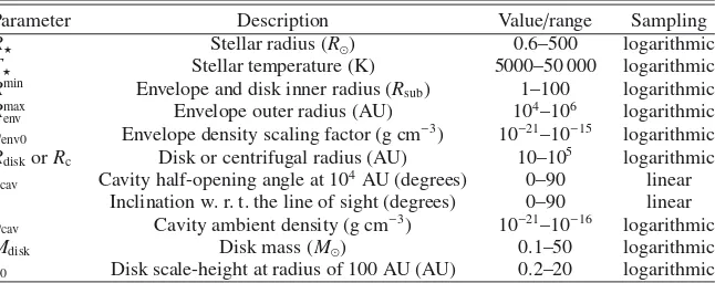
Table 4.Assumed ranges for model parameters as input to the genetic search algorithm.
Parameter Description Value/range Sampling
R Stellar radius (R) 0.6–500 logarithmic
T Stellar temperature (K) 5000–50 000 logarithmic
Rmin Envelope and disk inner radius (R
sub) 1–100 logarithmic Rmax
env Envelope outer radius (AU) 104–106 logarithmic ρenv0 Envelope density scaling factor (g cm−3) 10−21–10−15 logarithmic RdiskorRc Disk or centrifugal radius (AU) 10–105 logarithmic θcav Cavity half-opening angle at 104AU (degrees) 0–90 linear i Inclination w. r. t. the line of sight (degrees) 0–90 linear ρcav Cavity ambient density (g cm−3) 10−21–10−16 logarithmic
Mdisk Disk mass (M) 0.1–50 logarithmic
h0 Disk scale-height at radius of 100 AU (AU) 0.2–20 logarithmic
forθcav, as radiative transfer effects only work to make the cav-ity look larger than it actually is. For instance, light can be scat-tered into the envelope making it look larger, whereas because the density of the cavity is constant, there is no definite edge of emission seen within the cavity. The largest half-opening angle possible, for an inclination of 90◦, was therefore 54◦at a radius of 10 000 AU.
4.3. Model fitting
As part of the genetic algorithm used here and described in Johnston et al.(2011), the models were fit to the data using the SED fitting tool ofRobitaille et al.(2007), whereAv, the exter-nal extinction, was a free parameter in the fit. The distance was set to be 3.33 kpc, and the visual extinctionAv was allowed to vary between 0 and 40 mag.
As described in Robitaille et al. (2007), the fitting auto-matically takes into account the different circular aperture sizes
when fitting the models. However, in the case of the ISO fluxes, the ISO apertures are not circular, so instead the fluxes were determined by computing images at the ISO wavelengths, and summing up the flux weighted by the slit transmission maps (found within the Observer’s SWS Interactive Analysis software, OSIA7) which give the transmission as a function of location on
[image:7.595.138.461.437.565.2]24.6and 104wide strips aligned with and perpendicular to the outflow axis, and normalising them to the total flux. To produce the convolved modelJ,HandKsband images, the model images were convolved with the FWHM of the 2MASS point-spread functions (PSF) for each band: 3.15, 3.23 and 3.42 for J,
HandKs bands respectively, which were determined by fitting Gaussian PSFs to stars in the observed images. The model im-ages shown in Fig.2are high signal-to-noise versions of the im-ages used for fitting.
For both the SED and profiles, the errors were reset to 10% before fitting if the uncertainty in the measured flux was<10%. This was done to take into account non-measurement errors such as variability. The combined reducedχ2for each model given as input to the genetic algorithm was calculated as
χ2
combined=χ2SED+χ2profiles (7)
where χ2
SED is the best-fitting reduced χ2 value for the SED alone, andχ2
profilesis the overall reducedχ2for the profile fits. 5. Results
5.1. Results of SED and image modelling
In this paper, we model AFGL 2591 as a single source; as we will show in Sect.5.2.2, the second brightest object in the re-gion VLA 1 does not significantly contribute to its infrared flux, therefore this is a reasonable approximation.
The genetic code was run three times – firstly with the model parameter ranges given in Table4 as input for all parameters, which will be referred to as the “envelope with disk” model, and secondly with the parameter ranges given in Table4for all pa-rameters except the disk mass and disk scale height at 100 AU,
Mdisk and h0, which were set to zero and were therefore not treated as model parameters. This second run will be referred to as the “envelope without disk” model. The envelope without disk model was run to ascertain whether the SED and images could be adequately produced without a disk, i.e. a simpler model which had two fewer parameters. For the envelope without disk model,
Rdisk will instead be referred to as the centrifugal radius of the envelope,Rc, as these two parameters are interchangeable in the models. The third run had exactly the same setup as the envelope with disk model, but was used to determine the repeatability of the experiment and any parameter degeneracies, and will be re-ferred to as the control model.
The genetic search algorithm codes were stopped after 28, 29 and 49 generations for the envelope with disk, without disk and control models respectively, when the convergence criterion was reached. This corresponds to 6545 models or 2940 CPU hours for the envelope with disk model, 6278 models or 3774 CPU hours for the envelope without disk model, and 10536 models or 3960 CPU hours for the control model.
The resulting SEDs and profiles of the best-fitting models for the envelope with and without disk runs are shown against the data in Figs.1 and3, and the model images are compared to the observed images in Fig.2. The parameters of the best-fitting models (i.e. the model in each run with the lowest overall
χ2value after convergence), are also given in Table5. The inter-stellar extinctionAV for the best-fitting models of the envelope
with disk, without disk and control runs was 0.0, 0.0 and 0.8 respectively.
The minimum reducedχ2for the best-fitting envelope with disk model is 14.9, and the corresponding value for the best-fitting without disk model is 18.7, therefore the model with a
disk provides a marginally better fit to the SED and profiles. Comparing the model SEDs to the data shown in Fig.1, it can be seen that they are qualitatively very similar, although the model with a disk fits the SED slightly better. This difference is partially caused by their disagreement in the mid-IR regime, where the without disk model does not follow the data as closely. Figure3 also shows very similar fits to the 2MASS image profiles for each model, however the without disk model fits some of the profiles marginally better, being more centrally peaked. We note that although the reducedχ2 for the best-fitting model with a disk is lower, and thus provides evidence that an envelope with an embedded disk describes the source better than a model with-out a disk, the difference is not large enough to prove this con-clusively. We note that neither model provides a good fit to the
JandHband profiles along the outflow axis. This is likely to be caused by the fact that the emission at these wavelengths is not dominated by the central source, but instead by scattered light in the surrounding medium, which in reality is highly non-uniform, as seen in Figs.2and7. Thus to reproduce the images more accu-rately, future modelling will have to take such inhomogeneities into account, for example the “loops” in the outflow cavity seen in the near-IR images (Preibisch et al. 2003).
To understand how well the parameters of AFGL 2591 were determined, we took the best-fitting models for each run and var-ied in turn each parameter across the original parameter ranges, while holding the other parameters constant. We then fit the re-sultant SED and images for each new model, and calculated their overall reducedχ2-values. From these we could therefore deter-mine theχ2surfaces in the vicinity of the the best-fitting model parameters and hence understand their uncertainties. Figure4 shows such a plot for each varied parameter, for all three runs. Firstly, we can see the best-fitting values and shape of theχ2 sur-faces for stellar radius and temperature are different for each run, which is due to a degeneracy between these parameters. Theχ2 surfaces for the stellar luminosity, which is a combination of these two parameters, is shown as a panel in Fig.4: this sur-face is very well defined and very similar for all runs, showing that fitting the SED allows this parameter to be accurately and non-ambiguously determined. In the next panel we show theχ2 surface for the parameter orthogonal to the stellar luminosity,
R2
T, is flat and thus poorly determined. Therefore the SED or
image profiles do not provide a handle on either the stellar ra-dius and temperature, only the stellar luminosity. Similarly, the envelope density scaling factorρenv0andRdiskorRcare degen-erate, as they both determine the envelope density, which can be seen from Eq. (2). The final two panels of Fig.4, show the or-thogonal parameter combinationsρenvR3c/2andρenvR−c2/3. Here ρenvR3c/2is similar between the three runs, and has a sharpχ2 sur-face, while the best-fittingρenvR−c2/3value changes by an order of magnitude. Thus we cannot uniquely determine these two pa-rameters from our modelling, but we can determine a parameter that combines these which governs the overall envelope density and mass,ρenvR3c/2.
Table 5.Parameters of the genetic algorithm best-fitting models.
Parameter Description Value for envelope Value for envelope Value for envelope with with disk model without disk model disk control model
R Stellar radius (R) 90 200 52
T Stellar temperature (K) 13 000 8900 18 000
Rmin Envelope and disk inner radius (R
sub) 2.9 3.4 4.3
Rmax
env Envelope outer radius (AU) 180 000 420 000 790 000
ρenv0 Envelope density scaling factor (g cm−3) 2.4×10⁻¹⁹ 1.1×10⁻¹⁸ 5.6×10⁻¹⁸
RdiskorRc Disk or centrifugal radius (AU) 35 000 9500 2700
θcav Cavity half-opening angle at 104AU (degrees) 16 20 49
i Inclination w. r. t. the line of sight (degrees) 59 46 54
ρcav Cavity ambient density (g cm−3) 2.1×10⁻²⁰ 2.0×10⁻²⁰ 1.0×10⁻²¹
Mdisk Disk mass (M) 14 . . . 16
h0 Disk scale-height at radius of 100 AU (AU) 11 . . . 11
L Stellar luminosity (L) 2.3×10⁵ 2.3×10⁵ 2.4×10⁵
ρenv0R3c/2 Envelope density parameter (g cm−3AU3/2) 1.6×10⁻¹² 1.0×10⁻¹² 8.0×10⁻¹³
The shape of theχ2 surface for the cavity densityρcav is vari-able at higher values, but always has its minimum at low values, between 10−21and∼2 × 10⁻²⁰ g cm−3. For the two runs which include a disk, theχ2surfaces of the remaining parametersMdisk andh0are almost flat across the sampled ranges, although they slightly prefer values close to the upper limit. However, forh0 theχ2rises steeply toward the upper limit of the parameter range after its minimum at 11 AU.
In the remainder of this section, we compare the results of our modelling to the recent results from other studies of AFGL 2591. Firstly, our modelling finds values of roughly 2−5 Rsub for the envelope and disk inner radius Rmin. Using Eq. (5), we findRsub=34−39 AU for the three best-fitting mod-els, and hence we expect values ofRmin ∼ 70–200 AU. This value is in agreement with the radius of the inner cavity adopted byJiménez-Serra et al.(2012), who in turn took this value from the disk of emission observed byPreibisch et al.(2003), likely to be tracing the inner rim of the envelope and disk. At 1 kpc, Preibisch et al. (2003) found the radius of this emission was 40 AU, which is thus 130 AU at 3.33 kpc.
We compare the maximum envelope radiusRmax
env to the re-sults of the JCMT line observations ofvan der Wiel et al.(2011), which were able to trace the largest envelope scales, with the maximum radius in their model set to 200 000 AU (scaled to 3.33 kpc). This is in agreement with our SED modelling results, which prefer large envelope radii, on the scale of several hun-dreds of thousand AU.
We find the cavity half-opening angleθcavto be poorly con-strained by our modelling, although we determined an upper limit for the cavity half-opening angle of 54◦in Sect. 4.2 (de-fined at 104 AU). Wang et al. (2012) adopted an opening an-gle of 60◦, and hence a half-opening angle of 30◦, in their modelling. The models used inJiménez-Serra et al.(2012) and van der Wiel et al.(2011) do not include an outflow cavity.
We find the inclination to prefer intermediate values, be-tween roughly 30−65◦. This is in agreement with the adopted inclination of 30◦ by Wang et al. (2012), who in turn used the value determined by van der Tak et al. (2006). However, Jiménez-Serra et al.(2012) found an inclination of 20◦by mod-elling the position–velocity diagram of combined emission from several lines. Thus, previous results appear to favour an inclina-tion which is slightly closer to face-on. As the inclinainclina-tions for the envelope with and without disk models were 59 and 46◦ respec-tively, we therefore adopted an inclination of 50◦to determine
several of the physical properties of the jet and outflow in Sect.6.1, as a compromise between these two values.
We found low cavity densities ρcav were preferred for all runs, with best-fitting values between 10−21 and ∼2 × 10⁻²⁰g cm−3. InWang et al.(2012) andvan der Tak et al.(1999), their model cavity densities were set to zero.
Our modelling found the mass of the disk to be on the or-der of 10−20M, whereas using 0.5 203.4 GHz dust contin-uum observationsWang et al.(2012) determined the disk mass to be ∼1−3 M. However, as the disk mass was one of the most poorly determined parameters by our modelling, and as the interferometric dust continuum observations ofWang et al. (2012) directly measure the column density and thus mass of the disk, without the intervening emission or scattering from the envelope, we suggest that the result ofWang et al.(2012) is more robust.
It was not possible to compare our best-fitting values for the disk scale-heighth0to the model ofWang et al.(2012), as they instead used a sin5θfunction to describe the vertical structure of the disk, whereθis the angle from the polar axis, as opposed to our Gaussian profile withz.
The best-fitting luminosity of AFGL 2591 is 2.3 × 10⁵ L
for both the envelope with and without disk models respectively, which is in agreement with previous results (2.1−2.5 × 10⁵L
at 3.33 kpc,Lada et al. 1984;Henning et al. 1990;Rygl et al. 2012).
The envelope density parameter ρenv0 R3c/2 is a proxy for the mass of the envelope, which dominates the total mass of the enclosed circumstellar material at large radii, as it describes the scaling of Eq. (2). We find the total mass of the envelope plus disk is 1200 M for the envelope plus disk model, and 2700M for the envelope without disk model. The total mass of gas associated with the region observed byMinh & Yang (2008) is 2 × 10⁴ M
Fig. 4.Plots of theχ2surface along the axis of each model parameter for each run, determined by varying each parameter while holding the other best-fitting parameters constant. Red dashed line: envelope without disk run, light blue line: envelope with disk run, and black line: control run.
ofJiménez-Serra et al.(2012) is 1M. Comparing this to our model we find an enclosed mass within 2700 AU of 0.1Mfor the model without a disk, and 1M for the model with disk. Therefore in the case where there is a disk, the enclosed masses are in agreement.
5.2. 3.6 cm and 7 mm continuum
Figure5presents the observed multi-configuration 3.6 cm image of AFGL 2591. Panel a) shows the entire region surrounding the
Fig. 5. a) Map of the 3.6 cm continuum emission surrounding AFGL 2591. Contours are -3, 3, 4, 5, 7, 10, 15, 20, 30, 40, 50. . . 100× rms noise=30μJy beam−1. Greyscale: –0.03 to 3.77 mJy beam−1(1.2× peak value). The synthesised beam is shown in the bottom left corner: 0.43×0.40, PA=43◦.b)Close-up of the 3.6 cm continuum emission
towards VLA 3. Contours, greyscale and beam as in panela).
of Fig.5. The 3.6 cm emission from VLA 3 is consistent with a compact core plus jet morphology. The dominant side of the jet extends to the east, with a deconvolved width and length of
<0.2and 1.2(<670 AU and 4000 AU at 3.33 kpc), position angle of∼100◦, and an opening angle (at a radius of 4000 AU) of<10◦derived from its deconvolved width and length. The east jet is resolved, ending in a “knot” at 20h29m24s.98+40◦1119.3 (J2000). There is also a smaller corresponding jet to the west, seen as a slight extension of the source in this direction. The morphology of VLA 3 is consistent with a jet-system which is approximately parallel to the larger-scale flow (observed by e.g.
Hasegawa & Mitchell 1995), and therefore these observations confirm the proposal ofTrinidad et al.(2003) that VLA 3 is its powering source.
Figure 6 shows the 7 mm multi-configuration image of the region surrounding AFGL 2591, in which only VLA 1 and VLA 3 were detected at this resolution. VLA 3 is compact, with a radius of<500 AU, and is only slightly resolved in this im-age, showing no evidence of the eastern jet seen in Fig. 5 at 3.6 cm, which may partially be due to the 7 mm images having almost twice the rms noise. However, the A array-only image ofvan der Tak & Menten(2005), which has a synthesised beam size of 43 by 37 mas, shows that the source is slightly extended to the south-west, in a similar direction to the counter-jet seen in the 3.6 cm image. This extension is also seen in our multi-configuration 7 mm image. Using VLBA water maser observa-tions,Sanna et al.(2012) found that this emission most likely arises from the outflow cavity walls, which the masers they ob-served were also found to trace.
Table6provides the measured positions, peak and integrated fluxes, as well as deconvolved sizes for the sources observed in the 3.6 cm (8.4 GHz) and 7 mm (43.3 GHz) images. These were measured using a custom-made irregular aperture photometry program, with which the integrated flux density was measured above 1 sigma. Uncertainties in the aperture fluxes were calcu-lated to be a combination of the uncertainty due to the image noise over the aperture, and the maximum VLA absolute flux error, which is 2% and 5% for 3.6 cm and 7 mm respectively. Similarly, the peak flux uncertainty was found by combining the 1 sigma flux density with the VLA absolute flux error. The de-convolved source size at the 3−σlevel was measured by taking the major axis of the source to be along the direction which it is most extended, to within a position angle of 10◦.
Figure7 compares the 3.6 cm emission from the region to the near-IR emission recorded in the Gemini North images. The five detected H
ii
regions line-up with several features in the near-IR image. Firstly, the peak of VLA 3 is coincident with that of the central source of AFGL 2591, at the apex of the one sided reflection nebula. VLA 1 is instead anti-correlated with the dif-fuse near-IR emission. This dent or cavity in the cloud can be seen more clearly in the K band bispectrum speckle interferom-etry image ofPreibisch et al.(2003). VLA 2 also appears to be coincident with the close binary discovered byPreibisch et al. (2003), and VLA 4 with a source in the Gemini North image at 20h29m24s.3+40◦1128(J2000; however this source is too faint to be seen in Fig.7). In addition, VLA 5 may be powered by the bright source at 20h29m23s.96+40◦1109.25 (J2000; which is the same source as 2MASS 20292393+4011105, previously mentioned in Sect. 3.2). The sources VLA 1 and VLA 3 are discussed in detail below.5.2.1. The central source of AFGL 2591, VLA 3
Figure8shows the SED in frequency space of the central source of AFGL 2591, VLA 3, in black error bars. The fluxes shown for VLA 3, which are taken from the literature and this work, are listed in Tables3 (forλ < 1 mm) and7 (forλ > 1 mm). At
λ >1 mm, fluxes have been listed from the observations with the largest availableuvcoverage.
[image:11.595.39.291.77.562.2]Table 6.Measured properties of the observed 3.6 cm (8.4 GHz) and 7 mm (43 GHz) continuum sources.
Source λ Peak position Peak flux Integrated flux Deconvolved PA
name (cm) (J2000) density (mJy beam−1) density (mJy) source size () (degrees)
VLA 1 3.6 20 29 24.59+40 11 15.0 3.14±0.07 80±1.6 4.9 ×4.0 120 0.7 20 29 24.580+40 11 14.50 0.46±0.06 64±3.2 1.8 ×1.6 90 VLA 2 3.6 20 29 24.52+40 11 20.1 0.45±0.03 5.2±0.11 2.5 ×2.3 110
0.7 . . . .
VLA 3 3.6 20 29 24.88+40 11 19.5 0.72±0.03 1.52±0.03 1.9× 0.84 90 0.7 20 29 24.882+40 11 19.45 1.8±0.11 2.9±0.14 0.35 ×0.26 50 VLA 4 3.6 20 29 24.32+40 11 28.0 0.39±0.03 0.99±0.02 1.1× 0.78 90
0.7 . . . .
VLA 5 3.6 20 29 24.00+40 11 10.3 0.15±0.03 10.9±0.22 4.4 ×2.9 0
[image:12.595.39.291.249.535.2]0.7 . . . .
Fig. 6.Map of the 7 mm continuum emission towards AFGL 2591.
Contours are –4, 4, 7, 10, 15, 20, 25, 30×rms noise=56μJy beam−1. Greyscale: –0.06 to 2.14 mJy beam−1(1.2×peak value). The inset panel shows a close-up of the 7 mm emission from VLA 3. The synthesised beam is shown in the bottom left corner of both images: 0.11×0.11,
PA=43◦.
greybody. However, as these fluxes are taken from interferomet-ric observations, it is likely that they only contribute a fraction of the actual flux. For instance,van der Tak & Menten(2005) note that their quoted 226 GHz continuum flux represents only 5% of the total flux, due to lack of shorter baselines. An arrow is shown on Fig.8representing this correction, which agrees well with the flux expected at 226 GHz from the fitted greybody.
Extrapolating this greybody to 7 mm, a flux of 2.3 mJy is expected, but the measured flux of VLA 3 at 7 mm is 2.9 mJy. However, it is likely that a portion of the 7 mm flux is due to ionized gas emission as well as dust emission, and a significant fraction of this combined emission is resolved out by the inter-ferometer. To estimate the contribution from dust emission at
Fig. 7.Three-colourJHK Germini-North image of AFGL 2591 over-laid with the 3.6 cm contours from Fig.5. Stretch of Gemini image:red, Kband: 150−2500 MJy sr−1; green,Hband: 150−500 MJy sr−1; blue, Jband: 40−80 MJy sr−1.
[image:12.595.311.557.260.539.2]Fig. 8. Radio-SEDs of AFGL 2591-VLA 3 and VLA 1. The SED of AFGL 2591-VLA 3 is show in black error bars, and the resolved fluxes of AFGL 2591-VLA 3 fromMarengo et al.(2000) are shown as red squares. Green squares show the fluxes of VLA 1 – errors are not shown as they are smaller than the markers. The black and green solid lines show greybody fits to the SEDs of AFGL 2591-VLA 3 between 100 and 850μm, and VLA 1 at mid-IR fluxes, respectively (see Sects.5.2.1
and5.2.2). The green dashed line shows the fit to the long-wavelength fluxes for VLA 1.
To measure the spectral indexα(whereSν ∝να) of VLA 3,
which may give further insight into the nature of the emission, the 3.6 cm and 7 mm data were re-imaged usinguvdistances which were common to both datasets, from 4.5 to 1037 Kλ, and the fluxes remeasured. The integrated fluxes were found to be 1.43±0.03 mJy for 3.6 cm and 3.3±0.17 mJy for 7 mm (which increased compared to the original 7 mm flux due to a reduc-tion in resolureduc-tion, so that fainter emission was brought above the noise level). Therefore the spectral index between 3.6 cm and 7 mm was found to be 0.5±0.02, where the quoted error in the spectral index is due solely to the photometric errors, similar to the spectral index expected for an ionized wind, 0.6. However, as this value is measured from only two fluxes, it is likely to be more uncertain than the photometric errors given. This spec-tral index is also an upper limit, as we estimate a fraction of the 7 mm flux is due to dust emission. By applying the commonuv
distance range above, we derive<0.51 mJy for the contribution from dust emission, and therefore>2.8 mJy from ionized gas emission. Using this lower limit for the ionized gas emission at 7 mm, we estimate the spectral index to be between 0.4 and 0.5.
5.2.2. VLA 1
Figure8shows the SED of VLA 1 as green squares. This source was detected in the mid-IR byMarengo et al. (2000), as well as at several radio frequencies, for which the fluxes are listed in Table7. The spectrum of VLA 1 appears to be flat at radio wavelengths, with a fitted spectral indexαof 0.0±0.03. The fitted power-law is shown as a dashed line. However, we first need to verify whether only a fraction of the flux of VLA 1 is be-ing recovered at each wavelength. The flux of VLA 1 measured in our 3.6 cm A-D array image is not larger than the fluxes mea-sured in the A array only images in previous works (A-D array: 80 mJy, this work; A array only: 82 mJy, 94 mJy,Tofani et al. (1995) andTrinidad et al.(2003) respectively). In fact, there is
Table 7.Overview of observed fluxes for VLA 1 to VLA 5.
Source Wavelength Integrated flux Ref.
name density (mJy)
VLA 1 6 cm 79±2.0 (1)
3.6 cm 80±1.6 (2)
7 mm 64±3.2 (2)
3.4 mm 87±1.4 (3)
2.83 mm 71±1.2 (3)
2.81 mm 76±15 (20%) (2) 2.7 mm 72±14 (20%) (2)
2.6 mm 93±2.5 (3)
18.0μm 7.96±0.8×10⁴ (4) 12.5μm 1.59±0.2×10⁴ (4) 11.7μm 1.84±0.2×10⁴ (4)
VLA 2 6 cm 3.61±0.72 (1)
3.6 cm 5.2±0.11 (2)
VLA 3 6 cm 0.4±0.1 (1)
3.6 cm 1.52±0.03 (2) 1.3 cm 1.57±0.4 (5)
7 mm 2.9±0.14 (2)
3.4 mm 29.5±0.8 (3) 2.83 mm 38.7±0.7 (3) 2.81 mm 71±14 (20%) (2) 2.7 mm 79±16 (20%) (2) 2.6 mm 52.9±1.5 (3) 1.3 mm ∼151±4.5 (3) 18.0μm 7.53±0.75 × 10⁵ (4) 12.5μm 7.45±0.75 × 10⁵ (4) 11.7μm 4.40±0.44 × 10⁵ (4)
VLA 4 6 cm 0.65±0.13 (1)
3.6 cm 0.99±0.02 (2) VLA 5 3.6 cm 10.9±0.22 (2)
References.(1)Campbell(1984a); (2) this work; (3)van der Tak et al.
(1999); (4)Marengo et al.(2000); (5)Trinidad et al.(2003).
a small decrease in the flux of VLA 1 for the largeruvcoverage data. Therefore it is likely that most of the flux from VLA 1 has been recovered by observations which are sensitive to scales up to 7, the largest observable angular scale of VLA A array ob-servations at 3.6 cm. This is the case for all of the interferometric fluxes shown for VLA 1, hence the calculated flat spectral index of VLA 1 is not likely to be due to instrumental effects. The ob-served spectral index is close to that expected from optically thin free-free ionized gas emission (α=−0.1).
[image:13.595.327.534.100.416.2]Fig. 9. Continuum emission towards AFGL 2591 at 106.7 and 110.5 GHz (∼2.8 and 2.7 mm respectively), shown in both contours and greyscale. The rms noise in the images is σ = 2.2 and 2.1 mJy beam−1 respectively. The greyscales extend from
−3×σto 65.5 and 54.0 mJy beam−1. Contours are at −3,3,4,5,7,10,15 and 20 × σ. The crosses show the positions of VLA 1 to 3. The synthesised beams are 4.9×4.1PA=−4.8◦ and 4.3 ×3.5PA=95◦respectively.
5.3.13CO, C18O and 3 mm continuum
This section details the properties of the dense molecular gas surrounding AFGL 2591 inferred from the C18O molecular line and millimetre continuum observations.
Figure 9 shows the continuum emission from the region at 106.7 and 110.5 GHz, or 2.81 and 2.7 mm, in both of the wide∼3 mm continuum bands observed. The morphology of the emission is similar to that seen in the millimetre continuum maps at various wavelengths presented byvan der Tak et al.(1999), van der Tak et al.(2006), and resolved further byWang et al. (2012). We found that the sources in the 3 mm images were systematically offset from the 3.6 cm peak positions, which we determined to be caused by inaccurate coordinates used for the phase calibrator MWC 349 in the mm observations. We therefore shifted the continuum and line maps by 0.89in RA and 0.18 in declination to agree with the 7 mm position of MWC 349 A reported in Rodríguez et al. (2007). In Fig. 9, the peak posi-tions of VLA 1 to 3 are shown as crosses. The main two sources that are detected are VLA 1 and VLA 3, but there is also ex-tended emission towards the position of VLA 2. Although the large uncertainties in the two measured 3 mm fluxes do not al-low calculation of accurate spectral indices for VLA 1 and 2 us-ing these values alone, the difference in the spectral index of the two sources can be seen from the difference in their relative brightnesses between the two images, indicating VLA 1 has a flat spectral index, and VLA 3 has a rising spectral index at shorter wavelengths. In addition, when we compared both images con-volved with the beam of the 106.7 GHz image, the morphology of the emission was very similar, apart from the clear difference in the flux of VLA 3. The sources were fit with 2D Gaussians using the CASA task imfit to find the fluxes, which are given in Table7.
Figure10presents C18O and13CO line profiles at the posi-tion of AFGL 2591-VLA 3. The13CO observations were miss-ing significant flux on extended scales which, in combination with self-absorption effects, is likely to be the cause of the dip in the13CO line profile seen in Fig.10. As there was a signifi-cant amount of missing flux in the13CO line, and the emission was distributed incoherently across the maps, it was not possible to interpret this emission. Therefore the13CO data will not be discussed further, however channel maps of the13CO emission are included in Figs.11and12.
Figure13presents channel maps of the C18O emission to-wards AFGL 2591 between –9.0 and –2.7 km s−1 (where – 5.7 km s−1is the rest velocity of the cloud), and Fig.14shows the C18O intensity-weighted first moment map. In both figures
Fig. 10.C18O (black line) and13CO (grey line) spectral profiles mea-sured at the position of AFGL 2591-VLA 3: 20h29m24.s88+40◦1119.5 (J2000).
the positions of VLA 1 through 3 are marked by crosses, how-ever in Fig.14, the position and size of VLA 1 at 3.6 cm is shown instead as a circle. A blue-shifted velocity feature can be seen in Fig.14to the west of VLA 3, and coincident with VLA 2, which decreases smoothly in velocity to the west VLA 3, ranging from –5.3 to –8.0 km s−1. This can be seen in the C18O channel maps (Fig.13), which also show that the shape of the emission be-comes narrower away from the line centre and towards the west. This is most obvious in the –7.7 and –8.0 km s−1 channels. In addition, Fig.14shows that there is a smaller intensity peak∼6 to the south of VLA 3. Here, the velocity instead decreases from northwest to southeast from approximately –5 to –6 km s−1.
[image:14.595.307.557.257.447.2]Hasegawa & Mitchell(1995) using single dish12CO observa-tions with 14.3resolution, which extends in velocity from –45 to 35 km s−1. Therefore, the observations presented here trace the higher density but comparatively lower-velocity gas, within a few km s−1of the line centre. To minimise confusion due to over-lap in velocity of various components, the contours in Fig.15 only show integrated C18O emission from –4.3 to –3.3 km s−1 (red) and –8.0 to –7.0 km s−1(blue).
6. Discussion
6.1. The jet and outflow from VLA 3
In Fig.15, the extrapolated direction of the ionized jet observed at 3.6 cm points directly through the red-shifted C18O contours to the bow-shocks seen in theKband image. Hence this out-lines a coherent picture in which the red-shifted outflow lobe of AFGL 2591 consists of a small-scale 4000 AU ionized jet that is part of a jet or wind extending out to∼0.4 pc where the flow terminates against the surrounding cloud as bow-shocks. However it is interesting to note that the position angle of the jet and bow shocks do not exactly align with that of the blue-shifted reflection nebula or the elongation of the blue-shifted outflow observed byHasegawa & Mitchell(1995). Therefore other stars in the vicinity, such as the powering star(s) of VLA 1, may be causing precession of the jet. If, as well as the emission lying along the position angle of the ionized jet, the clump of emis-sion at 20h29m26s.7+40◦1123 (J2000) is also included, these three clumps may be tracing an arc of emission describing the densest parts of the red-shifted outflow lobe, created as the jet precesses. If so, the extent of these clumps corresponds to an ob-served opening angle of∼40◦at their distance from the source,
∼0.4 pc. At the same distance, the observed blue-shifted outflow lobe is larger with an opening angle of∼60◦. The opening an-gles of the biconical outflow observed byJiménez-Serra et al. (2012) and the blue shifted outflow cone observed bySanna et al. (2012), on scales<2or<6700 AU, are∼90–110◦. The larger observed opening angles on smaller scales suggests that the out-flow cavity can not be described by a cone with a constant open-ing angle, but is instead better described by a power-law cavity similar to that used in our radiative transfer models.
Several suggestions regarding the nature of the mm and cm continuum emission from VLA 3 have been made by previous studies, including a core-halo H
ii
region, an ionized wind with a dust disk (Trinidad et al. 2003), or emission from a spheri-cal gravitationally confined Hii
region (van der Tak & Menten 2005). At 3.6 cm, the deeper observations presented here clearly show that as well as a central compact core, the source also ex-hibits a non-spherical jet-like morphology. Therefore, we cal-culate several properties of the emission below, assuming it originates from a jet.Without assuming a specific ionization mechanism, the mass loss rate of the jet can be estimated using the model ofReynolds (1986), which describes the emission from a partially optically thick ionized jet (his Eq. (19)):
˙
M
10−6Myr−1 =9.38×10
−2
υ
100 km s−1 1 x0 μ mp × Sν mJy ν 10 GHz
−α 0.75
d
kpc
1.5 ν
m
10 GHz
−0.45+0.75α
× θ0.75 T 104K
−0.075
(sini)−0.25F−0.75 (8)
whereυis the velocity of the jet,x0 is the ionization fraction; μ/mp is the mean particle mass per hydrogen atom of the
ion-ized material, given by 1/(1+x0); Sν is the observed flux at the frequencyν;αis the spectral index;dis the distance to the source;νmis the turn-over frequency below which the emission
becomes optically thick;θis the opening angle of the flow, de-fined as the ratio of the projected width to the radius at the base of the jet; T is the temperature of the ionized gas;iis the in-clination measured from the line-of-sight andFis a function of the spectral index and the dependance of optical depth on radius (seeReynolds 1986, Eq. (17)).
Assuming an isothermal, uniformly ionized jet with a density gradient of ρ ∼ r−2; υ = 500 km s−1 for the velocity of the jet, found for the blue-shifted HH objects towards AFGL 2591 (Poetzel et al. 1992);x0 =0.1 (commonly found for low-mass sources, e.g.Bacciotti & Eislöffel 1999);vm = 50 GHz; θ ∼ 0.2/1.2, the ratio of the maximum deconvolved width to the maximum radius;T =104K ; a spectral index between 0.4 and 0.5; andi=50◦, taken from the results of the SED and near-IR image profile modelling presented in Sect.5.1;Fwas found to be between 2.3 and 1.8, and the mass loss rate of the jet observed at 3.6 cm was therefore determined to be in the range 0.77−1.0× 10⁻⁵M
yr−1.
This value is approximately a thousand times larger than the jet mass loss rates seen for low-mass protostars, which are com-monly found to be on the order of 10−8M
yr−1(e.g.Podio et al.
2006). The mass loss rate in this jet can also be compared to the mass loss rate of the small-scale red-shifted molecular flow ob-served byHasegawa & Mitchell(1995) in12CO(J=3−2), which corresponds well to the position and direction of the outflow lobe suggested by the ionized jet, red-shifted C18O emission and bow shocks discussed in Sect.5.3. For their optically thick case, Hasegawa & Mitchellfind a mass loss rate of 6.3×10⁻⁵Myr−1 at 1 kpc corresponding to 7.0 ×10⁻⁴M
yr−1at 3.33 kpc. Multiplying the ionized jet mass loss rate by the velocityυ, the momentum rate in the jet is 3.9−5.2×10⁻³M
yr−1km s−1, which is very similar to the momentum rates determined by Hasegawa & Mitchell(1995) for both the large and small scale red-shifted12CO outflows (7.7 and 7.4 ×10⁻³ M
yr−1km s−1 at 3.33 kpc with i = 50◦, scaled from 7.5 and 7.2 × 10⁻⁴ M
yr−1 km s−1 at 1 kpc withi = 45◦). Thus the jet it-self would have very close to the required momentum to drive the observed larger scale red-shifted outflow.
The ionization mechanism of the jet can be modelled as a plane-parallel shock in a homogeneous neutral “stellar” wind (e.g.Curiel et al. 1989;Anglada 1996). The momentum rate ˙P
of the jet can be expressed as:
˙
P Myr−1km s−1
= 3.13×η10−4
Sνd2
mJy kpc2
υ
200 km s−1
0.32
× T
104K
−0.45 ν
5 GHz
0.1 τ
1−e−τ
(9) whereηis the shock efficiency or ionization fraction, found to be∼0.1 for low-mass sources (e.g.Bacciotti & Eislöffel 1999),
υ is the initial velocity of the stellar wind or jet, taken to be
500 km s−1, andτis the optical depth of the emitting gas. Here, the fluxSνis measured at 3.6 cm. The optical depth can be
de-termined using Eq. (6) ofAnglada et al.(1998):
α=2+ln
(1−e−τ1)/1−e−τ1(ν1/ν2)2.1
ln (ν1/ν2) ·