This is a repository copy of
Predicting Multimedia Traffic in Wireless Networks: A
Performance Evaluation of Cognitive Techniques
.
White Rose Research Online URL for this paper:
http://eprints.whiterose.ac.uk/116429/
Version: Accepted Version
Proceedings Paper:
Sarigiannidis, P., Aproikidis, K., Louta, M. et al. (2 more authors) (2014) Predicting
Multimedia Traffic in Wireless Networks: A Performance Evaluation of Cognitive
Techniques. In: The 5th International Conference on Information, Intelligence, Systems
and Applications, IISA 2014. IISA 2014, The 5th International Conference on Information,
Intelligence, Systems and Applications, 7-9 July 2014, Chania, Greece. IEEE . ISBN
978-1-4799-6171-9
https://doi.org/10.1109/IISA.2014.6878802
© 2016 IEEE. Personal use of this material is permitted. Permission from IEEE must be
obtained for all other users, including reprinting/ republishing this material for advertising or
promotional purposes, creating new collective works for resale or redistribution to servers
or lists, or reuse of any copyrighted components of this work in other works.
[email protected] https://eprints.whiterose.ac.uk/ Reuse
Unless indicated otherwise, fulltext items are protected by copyright with all rights reserved. The copyright exception in section 29 of the Copyright, Designs and Patents Act 1988 allows the making of a single copy solely for the purpose of non-commercial research or private study within the limits of fair dealing. The publisher or other rights-holder may allow further reproduction and re-use of this version - refer to the White Rose Research Online record for this item. Where records identify the publisher as the copyright holder, users can verify any specific terms of use on the publisher’s website.
Takedown
If you consider content in White Rose Research Online to be in breach of UK law, please notify us by
Predicting Multimedia Traffic in Wireless Networks:
A Performance Evaluation of Cognitive Techniques
Panagiotis Sarigiannidis
Konstantinos Aproikidis
Malamati Louta
Pantelis Angelidis
Department of Informatics and Telecommunications Engineering University of Western Macedonia
Kozani, Greece
Contact E-mail: [email protected]
Thomas Lagkas
The University of Sheffield International Faculty CITY College
Thessaloniki, Greece
Abstract—Traffic engineering in networking is defined as the process that incorporates sophisticated methods in order to ensure optimization and high network performance. One of the most constructive tools employed by the traffic engineering concept is the traffic prediction. Having in mind the hetero-geneous traffic patterns originated by various modern services and network platforms, the need of a robust, cognitive, and error-free prediction technique becomes even more pressing. This work focuses on the prediction concept as an autonomous, functional, and efficient process, where multiple cutting-edge methods are presented, modeled, and thoroughly assessed. To this purpose, real traffic traces have been captured, including multiple multimedia traffic flows, so as to comparatively assess widely used methods in terms of accuracy.
Keywords—extrapolation; automata; markov chains; prediction; wireless networks;
I. INTRODUCTION
Modern services and applications require a robust net-work framenet-work, including many intelligent, cognitive, and sophisticated processes and procedures, in order to reach the maximum of their capabilities. Latest wireless standards incorporate intelligent functionality, dynamic allocation, and expanded control; however they entail an efficient supportive suite of surrounded protocols and algorithms. For instance, semi-persistent scheduling in Long Term Evolution (LTE) net-works involves dynamic scheduling in allocating burst grants in voice packet transmission. Moreover, traffic engineering emerges as a beneficial and supportive framework towards ensuring high levels of network performance. Among others, traffic engineering adopts prediction/estimation techniques in order to provide various decision processes with complete or insightful picture on critical information. Multitude prediction tools have been developed for providing forecasting in wireless networks [1], cognitive networks [2], and wired networks, such as optical networking [3].
In general, a prediction tool is used to forecast a sequence of time series. In the context of wireless networking, the values represented by the series may be attached to various performance parameters such as a) packet size. b) interarrival time, c) number of users, d) duration of a sleeping period, e) burstiness, and f) signal or noise levels. In essence, by
applying a prediction process an a priori knowledge is ob-tained regarding a specific network parameter. For example, by forecasting the packet size and the interarrival time of users’ traffic requests the efficacy of the computed decisions could be thoroughly improved even totally optimized if the prediction process is quite accurate. In wireless environments, where the main goals are the low user’s perceived latency, due to application sensitivity, and the high channel utilization, due to bandwidth limitations, the utilization of a rigorous prediction tool could be extremely beneficial. In this way, modern wireless networks could cope with the proliferation of cellular network, accompanied with the vast growth of users involved, as well as the fast penetration of bandwidth-demanding Internet services.
Following the definition given in [4], traffic prediction is the task of retrieving the past traffic requests in deducing what the future bandwidth requests will be. Accordingly, traffic prediction can positively affect the network performance by allowing more efficient decisions. For example, in a time instance, a decision component can allocate surplus bandwidth from users that will not use it to users that really need it if it is aware of users’ bandwidth requests in advance. Thus, the channel utilization is improved since the wasted bandwidth, due to idle/inactive users, is properly exploited and user latency is reduced due to the fact that the bandwidth requests of active users are faster satisfied. However, the applied prediction method is necessary to be accurate enough inducing low error rate. It is obvious that an inefficient traffic estimation could lead to performance impairments such as unfair schedule, under-utilization, and high delays.
In this work, the cognitive capabilities of several cutting-edge prediction methods are identified. In order to stimulate the solidity of our research, we apply these methods to real traffic traces obtained from a Worldwide Interoperability for Microwave Access (WiMAX) infrastructure. Yet, the obtained traces belong to various multimedia flows such as Voice over IP (VoIP) and live streaming, offering even more credibility in our research findings. The contributions of this work are summarized as follows:
• It presents the most popular, efficient, and effective prediction tools focused on the traffic prediction.
• It thoroughly assesses the prediction tools in terms of accuracy and effectiveness.
• It incorporates a real-time prediction framework by using real traffic traces captured during actual multi-media data delivery.
• It identifies each tool’s merits and inefficiencies. Fur-thermore, it infers about the most applicable predic-tion tool regarding multimedia traffic of a broadband wireless network.
The remainder of this paper is organized as follows. Section III describes the adopted prediction tools in detail, while Section II outlines previous work in communication networks. Section IV presents evaluation results accompanied by detailed comments. Finally, Section V concludes this paper.
II. RELATEDWORK
Considering modern communication networks and proto-cols, three of the most popular and effective cognitive pre-diction tools are a) interpolation and extrapolation, b) Markov chains, and c) learning automata (LAs).
Interpolation and extrapolation methods are quite popu-lar in approximating unknown functions. Furthermore, they are employed to dynamically determine the most appropriate downlink-to-uplink width ratio in accordance to traffic de-mands in WiMAX systems [5], facilitate the spectrum access in cognitive radio networks [6], estimate channel characteristics in Multi-User Multiple Input Multiple Output (MU-MIMO) systems [7], and approximate the item demand probability distribution function in wireless push systems [8].
LAs have found use in communication networks, espe-cially in wireless networking. In underwater acoustic wireless networks the authors in [9] investigate the data dissemination and the high latency problem by enhancing an adaptive push system with a LA component. A paradigm of developing traffic engineering using LA can be found in [10]. Lastly, in [11] the BaseStation (BS) of a WiMAX access network is strengthened by utilizing a LA in order to improve the bandwidth allocation process.
Models built by Markov chains are quite popular in com-munication and networking. In [12] a framework that performs Quality of Experience (QoE) estimation and prediction using passive probing mechanisms is presented, while in [3] a Hidden Markov Chain (HMC) is designed to predict individual Quality of Service (QoS) features is suggested. The authors in [13] introduced a Markov renewal process for both mobility modeling and predicting in wireless networks. The work in [14] inaugurates an efficient content sharing scheme for smartphone networks. Lastly, a new algorithm for predicting audio packet playout delay for VoIP conferencing applications is implemented in [15].
III. PREDICTIONTOOLS
A. Extrapolation Techniques
Both interpolation and extrapolation methods are quite popular on fitting smooth continuous functions through dis-crete data. Interpolation uses actual scattered data to estimate
unknown values between the lower and the upper value of the actual set. On the other hand, extrapolation estimates values beyond the limits of the actual set. For example, assuming that for the time series of x = [1.2,2.3,3.7,4.3,5.5] the values of function F are F = [5.2,4.6,3.4,2.1,0.5], the aim of interpolation is to estimate the value of F given that 1.2≤x≤5.5, e.g., the value of F(3.9). On the contrary, the extrapolation technique intends to predict the F value when x >5.5orx <1.2, e.g., the value ofF(6.1).
In the context of traffic prediction the extrapolation method is functional since it allows the prediction of future values in advance. Among other interesting extrapolation techniques, the
Lagrangian Polynomials and the Spline Curves are the most attractive ones.
Maybe the most straightforward way to extrapolate data is the Lagrangian Polynomials. Given a set of historical data, the method of Lagrangian Polynomials forms a sum of polynomials in order to fit the unknown function that generated the actual (historical) data. Consider an actual set ofF(x1), F(x2), ..., F(xn)values for a given set ofxvalues,
x1, x2, ..., xn. These values are real and have been measured
in the context of an experiment. The Lagrangian Polynomial
forms the polynomial R(x) aiming at fitting the unknown function F, whereR(x) =Pn
j=1Rj(x). The functionRj(x)
is further defined as Rj(x) = F(xj)Qnk=1,k6=j x−xk
xj−xk. It is
obvious that the estimated polynomial R(x) passes through the known values trying to extend the form of the estimated functionF. In addition, the polynomialR(x)has a degree of at most n−1.
Polynomials of high degrees may present great deviations resulting in high estimation error. Spline Curves, or simply
Splines, constitute piecewise polynomial functions that com-bine simplicity, in terms of computing parameters, and flexibil-ity, in terms of smoothness and easiness on handling arbitrary functions. In essence,Splines are piecewise polynomials with pieces that are smoothly connected together.
One of the most interesting advantages of Splines is the low complexity, since they keep the computational re-quirements low compared to other interpolation techniques that include complex numerical calculations, involving higher degree curves. The Cubic Spline is further popular, since it offers minimum curvature property, high-quality fitting, simple representation, and smoothness.
Given a set ofn+ 1knots, that is historical (actual) values, each pair of successive knots(xj, xj+1), j= [1,2, ..., n, n+1],
corresponding toF(xj), F(xj+1), defines aSpline. This means
that a Spline fits a set ofnth-degree polynomials between each
pair of knots. The approximation function S(x)is defined as follows:
S(x) =
S1(x) if x1≤x≤x2
S2(x) if x2≤x≤x3
. . . .
Sn(x) if xn ≤x≤xn+1
(1)
The Sj(x) denotes a third (cubic) degree polynomial
be-tween the jth knot, that is (x
j, xj+1), j = [1,2, ..., n]. It has
Sj(x) =aj(x−xj)3+bj(x−xj)2+cj(x−xj) +dj (2)
Theaj, bj, cjanddjparameters are determined as follows:
aj=
Sj+1−Sj
6(x−xj+1)
, bj=
Sj
2
cj=
F(xj+1)−F(xj)
(x−xj+1)
−2(x−xj+1)Sj+ (x−xj+1)Sj+1 6
dj =F(xj)
BothLagrangian Polynomial andCubic Splinetechniques are incorporated and assessed in this work. The function of the extrapolation techniques in order to be able to predict network traffic is modeled as follows. The time domain is divided into discrete time instances, T = [0,1, ...]. Each arrival represents a time instance, i.e., the first arrival triggers time instance T = 0, the second happens in T = 1 etc. On the one hand, each arrival generates an integer value corresponding the data packet size in [64,1518], in terms of Bytes, since an Ethernet network is considered. Hence, the extrapolation intends to predict the (next) packet size at time T = tn+1, known the actual values of all previous arrivals
0≤T ≤tn. In other words, the extrapolation method tries to
estimate the actual value of Fsize(x
tn+1), i.e., actual packet
size, by forming the polynomials Rsize
tn+1(x)and S size tn+1(x)for
Lagrangian PolynomialsandSplinesrespectively. In a similar way, the estimation of the (next) arrival time in sec follows the same structure in time domain; however the polynomials Rtime
tn+1(x) and S time
tn+1(x) indicate (arrival) time values based
on the (arrival) times of the past given by the actual function Ftime(x
tn+1).
B. Markov Chains
Markov processes provide very flexible, powerful, and efficient means for the description and analysis of dynamic (computer) system properties. Markov processes constitute a special subclass of stochastic processes. In particular, a stochastic process provides a relation between the elements of a possibly infinite family of random variables. A series of random experiments can thus be taken into consideration and analyzed as a whole [16].
Considering a number ofnobservations obtained from an experiment, an actual set of F(x1), F(x2), ..., F(xn) values
for a given set ofxvalues,x1, x2, ..., xnis defined. In general,
a stochastic process,Xtis defined as a set of random variables
in the time domain, t∈ T, whereT ⊆R+ = [0,∞]. Taking
into account that our objective is to predict the (future) values ofF, the problem is formulated in estimating the values ofXt
when t > tcurrent wheretcurrent is the current time instance.
The stochastic process incorporates a state spaceB which represents the set of all possible values ofXt. In our case, the
state space B represents all possible values of the underlying functionF. In addition, we consider a countable time param-eter T resulting in a discrete-parameter process, thusT obeys to N0. For instance, if F(x) generates the number of users connected to a wireless BS at timex, thenF(x)∈[0, n], where
n is the maximum accepted number of users in the BS. The state space B in this case is defined as B = [B1, B2, ..., Bn]
indicating the number of connected users as a distinct state.
In the light of the aforementioned observations, a stochastic process Xt defines a Markov process if for all t, t1 < t2 <
... < tn and all states ofB theXtn+1 depends only on the last
value Xtn and not on the earlier values:
P(Xtn+1 ≤Bn+1|Xtn =Bn) (3)
In predicting the packet size, each state corresponds to all possible values, i.e., Bsize = [64,65, ...,1518]. However,
predicting (arrival) times is not straightforward, because the actual values are real numbers. To remedy this difficulty, we normalize the allowable arrival times in equally divided spaces of 0.2 sec. Hence, Btime = [0.2,0.4, ...]. For each time instance t, the actual state is denoted as qsize
t (qtimet ).
Since each state corresponds to a specific observation notation, the specifications and the observation features,Otsize/time, are
defined below:
P(Osizet =kzsize|qtsize=Bzsize) (4)
P(Otimet =ktimey |qtimet =Bytime) (5)
where 1 ≤ z ≤ 1455, 1 ≤ y ≤ 301, while ksize
1 =
64, ksize
2 = 65, . . . k1455size = 1518, and ktime1 = 0.2, ktime2 =
0.4, . . . ksize
301 > 60. The special value of k301size is associated
with (arrival) time values larger than 1 min. The state transition probability distribution is described by the following equation:
asizei,j =P
qtsize′ =B
size
j |qtsize=Bsizei
(6) atimem,n =P
qttime′ =B
time
j |qttime=Btimei
(7)
where 1 ≤ i, j ≤ 1455 and 1 ≤ m, n ≤ 301.asize
i,j (atimem,n)
denotes the transition probability from state i (m) to state j (n), and i, j (m, n) symbolize the length of the packet arrived (arrival time) at (between)tandt′, respectively, while t′denotes the next time instance. Each state stores the number transitions for all other states. Finally, the most frequent transition from the actual one is selected by the prediction model as the next (estimated) action.
C. Learning Automata
of the major merits the LAs exhibit is their low computational complexity.
An LA continuously interacts with the random operating environment so as to find among a set of actions the one that minimizes the average penalty the system receives by the environment [17]. Assuming a set of nallowable actions, e(1), e(2), ..., e(n)this process can be modeled considering a probability distribution vector, Li, i= 1,2, ..., n, which keeps
and calculates the probability of each action e(j). In order to preserve model’s consistency, it holds that Pn
i=1Li = 1.
The operation of predicting is based on a specific process which is incorporated by the prediction module. This process is called probability updating algorithm and its functionality is inherited by the features of the reinforcement learning. The time is divided into cycles (time instances), where the LA in each cycletutilizes the feedback received by the environment in the previous cyclet−1to perform a prediction concerning the next cycle t + 1. Upon performing the prediction, the LA receives (again) a feedback, as a result of the action performed, which is used in order to update the probability distribution vector. In general, the probability of the actual action is favored, while all others are slightly reduced. To this end, the optimal action is distinguished from the action set by emerging as the most probable, and therefore preferable, action to the environment.
The probability updating algorithm may have multiple versions according to the subtle features of the environment. For example, the Linear Reward-Penalty (LR-P) scheme could be followed, where the LA selects an action from the pool and, after reception of a favorable response for the action that was selected, the corresponding probability of selecting this action again is increased, whereas after reception of an unfavorable response the probability of selecting this action again is decreased. On the other hand, the Linear Reward-Inaction (LR-I) scheme involves inaction upon the reception of an unfavorable response regarding the probability of the selected action. In this paper, the LR-I scheme is adopted and the update algorithm is structured as follows, where e(o),1≤o≤ndenotes the action the environment responds:
Li(t+ 1) =Li(t)−V(Li(t)−u),∀e(i)6=e(o) (8)
Li(t+ 1) =Li(t) +V
X
i6=o
(Li(t)−u),ifi=o (9)
The V parameter constitutes the convergence rate of the learning process. A larger V leads to faster convergence since the update probability process is accelerated but causes higher fluctuation. Theuparameter simply stands to avoid the probabilities from taking zero values. Hence, it usually receives a minimum value, e.g.,10−5
.
Here, the allowable actions
esize(1), esize(2), ..., esize(1455) and
etime(1), etime(2), ..., etime(301) denote all possible values
of packet length, i.e.,[64,1518], and all possible (normalized) values if arrival time, i.e., [0.2,60]. Initially, all probabilities, i.e., Lsize
i (Ltimei ) are received the initial value of 1/1455
(1/301).
1000 2000 3000 4000 5000 6000 7000 8000 9000 10000 2
3 4 5 6 7 8 9
10x 10
-3
Cycles
M
ea
n
e
rr
o
r
ra
te
[image:5.612.341.542.54.223.2]Cubic Splines Lagrangian Polynomials
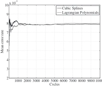
Fig. 1. Lagrangian Polynomials vs. Cubic Splines in terms of mean error rate.
IV. PERFORMANCEEVALUATION
1) Environment: In order to provide a robust evaluation en-vironment, we engaged real WiMAX multimedia traffic traces stemming from a WiMAX access network during sessions between a BS and a Mobile Station (MS). The captured traffic corresponds to the downlink direction, i.e., the traffic delivered by the MS from the BS. The captured traffic streams were obtained using the Wireshark tool. Two traffic streams have been utilized: a) a VoIP session between a BS and a MS using the User Datagram Protocol (UDP) and the Skype application and b) a Real Media Streaming application based on Transmission Control Protocol (TCP). In each traffic stream two objectives are set, namely a) to predict the packet size in bytes and b) to predict the time of the next (packet) arrival (between two successive arrivals) in seconds. The simulator has been implemented in Matlab, while for each traffic stream three traffic parameters have been used: a) the packet serial number (ID), b) the packet size in Bytes, and c) the arrival time.
The assessment is based on accuracy in terms of mean error rate. In particular, the mean error rate is defined as follows:
E=|ActualV alue−P redictedV alue|
T otalP ossibleV alues (10)
Concerning the VoIP application, the MS produced an average traffic of 0.038 Mbps, while the average packet size is equal to 1372 Bytes. The streaming application generated an average traffic of 0.04 Mbps having an average packet size of 121 Bytes. A number of 10000 samples, known as cycles, for both packet and interarrival time prediction has been retrieved. For each prediction tool a learning period is initiated, where the prediction module learns without providing output. The default value of the learning period duration is the 10% of the total cycles. Common values ofV anduare0.1and10−5
and these are adopted as default values for the present evaluation.
1000 2000 3000 4000 5000 6000 7000 8000 9000 10000 0.05
0.1 0.15 0.2 0.25
Cycles
M
ea
n
e
rr
o
r
ra
te
[image:6.612.343.544.54.215.2]Training Period of 10% Training Period of 30% Training Period of 1%
Fig. 2. Hidden Markov Chains evaluation in terms of training period.
1000 2000 3000 4000 5000 6000 7000 8000 9000 10000 0.1
0.15 0.2 0.25 0.3 0.35 0.4
Cycles
M
ea
n
e
rr
o
r
ra
te
[image:6.612.71.277.54.203.2]V = 0.1 V = 0.01 V = 0.001
Fig. 3. Learning Automata evaluation in terms of convergence speed.
1000 2000 3000 4000 5000 6000 7000 8000 9000 10000 0.2
0.4 0.6 0.8 1 1.2 1.4
Cycles
M
ea
n
e
rr
o
r
ra
te
Extrapolation HMC LA
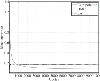
Fig. 4. Streaming session. Mean error rate on predicting the packet size in Bytes.
have been comparatively evaluated. Fig 1 depicts the results of this comparison. Initially both techniques experience high error rates due to the fact that the prediction process endeavors to learn the most frequent, and therefore, the appropriate packet size values. After 2000 cycles both techniques converge presenting an almost stable error rate of 8·10−3
. In general, similar accuracy is observed for both techniques. However, the
Cubic Splinestechnique seems to offer slightly more accurate predictions, due to its ability to smoothly engaging
polynomi-1000 2000 3000 4000 5000 6000 7000 8000 9000 polynomi-10000 0.1
0.2 0.3 0.4 0.5 0.6 0.7
Cycles
M
ea
n
e
rr
o
r
ra
te
[image:6.612.72.276.239.387.2]Extrapolation HMC LA
Fig. 5. Streaming session. Mean error rate on predicting the arrival time in sec.
1000 2000 3000 4000 5000 6000 7000 8000 9000 10000 0.2
0.4 0.6 0.8 1 1.2 1.4
Cycles
M
ea
n
e
rr
o
r
ra
te
Extrapolation HMC LA
Fig. 6. VoIP session. Mean error rate on predicting the packet size in Bytes.
1000 2000 3000 4000 5000 6000 7000 8000 9000 10000 0.2
0.4 0.6 0.8 1 1.2 1.4
Cycles
M
ea
n
e
rr
o
r
ra
te
Extrapolation HMC LA
Fig. 7. VoIP session. Mean error rate on predicting the arrival time in sec.
als, hence it is indicated as the representative technique of the extrapolation method.
[image:6.612.342.542.258.421.2] [image:6.612.71.276.421.583.2] [image:6.612.342.542.456.618.2]shown where the learning period takes three different values, i.e., 100, 1000, and 3000. Once more the captured data of the streaming session were utilized in terms of data packet size. The results do not reveal anything special regarding the performance of HMC. In any case, the error rate reaches 0.07 approximately, hence it can be deduced that HMC is quite well on predicting the length of data packets regarding a streaming session. Another aspect raised has to do with the learning capability of the HMC tool. Indeed, Markov chains are able to adapt fast in the environment, offering immediate positive results.
In Fig 3 the efficiency of the LA tool is inspected. Again, the set of packet size data of the streaming session was fed to the model. Here, the parameter under evaluation is the convergence speed V which determines the impact of the probability updating algorithm in Eq. (8). It is obvious that the value ofV = 0.1is the most effective one. This is attached to the fact that predicting data packet length is a job that could allow a fast convergence since identical data packets are often repeated, hence the prediction module has the potential to learn quickly.
The next two figures, namely Fig 4 and Fig 5 provide an evaluation comparison between all prediction tools when the data packet size and the arrival time is estimated respectively. As previously, a total of 10000 samples have been utilized. The default value of the learning period is 1000 cycles. Two major aspects are raised by observing the Fig 4: a) the extrapolation technique seems to be the most efficient and b) all methods offer low levels of error rate, i.e., below 10%. Maybe, the superiority of the extrapolation method is a combination of smooth fitting and good matching due to the nature of the data under prediction. Furthermore, the above observations are yet enhanced by noticing that both HMC and LA require some time to converge. Similar conclusions are drawn by examining the Fig 5. It is worth mentioning that the obtained error level of the extrapolation method is quite low, while it converges almost immediately. LA present the highest levels of error, fact that stems from its functional operation; it often changes its optimal decision.
Lastly, Fig 6 depicts the prediction results on estimating the data packet size using the VoIP session as input. Accordingly, in Fig 7 the arrival predictions are illustrated. The observation of these figures lead to three critical remarks. First, the extrapolation technique looks as the most promising one since it provides accurate predictions for both data packet size and arrival time. Thus, it is capable of adequately estimating the main parameters of a (multimedia) traffic flow. Second, the HMC tool presents a fair error rate, below 10%. Third, the use of the LA tool is deemed as good enough, however it fails to ensure quite precise estimations as the extrapolation techniques does. In a nutshell, the usage of the extrapolation tool is indicated for multimedia traffic estimations based on our findings.
V. CONCLUSION
Three heterogeneous, cognitive prediction frameworks were modeled, presented, and evaluated on the basis of multi-media traffic prediction. All techniques utilized, namely extrap-olation, Markov chains, and learning automata, demonstrated
notable estimation capabilities on predicting critical traffic parameters such as the data packet length and the arrival time. Our findings indicated that the usage of the extrapolation technique seems the most effective due to its ability to offer smooth fitting and fast learning ability.
REFERENCES
[1] H. Abou-zeid, H. Hassanein, and S. Valentin, “Energy-efficient adaptive video transmission: Exploiting rate predictions in wireless networks,” pp. 1–1, 2014.
[2] X. Xing, T. Jing, W. Cheng, Y. Huo, and X. Cheng, “Spectrum pre-diction in cognitive radio networks,”Wireless Communications, IEEE, vol. 20, no. 2, pp. 90–96, April 2013.
[3] P. Sarigiannidis, “Applying quality of service prediction in wdm optical networks,” in MELECON 2010 - 2010 15th IEEE Mediterranean
Electrotechnical Conference, April 2010, pp. 1406–1410.
[4] D. Katsaros and Y. Manolopoulos, “Prediction in wireless networks by markov chains,” Wireless Communications, IEEE, vol. 16, no. 2, pp. 56–64, April 2009.
[5] P. Sarigiannidis, M. Louta, and A. Michalas, “On effectively determin-ing the downlink-to-uplink sub-frame width ratio for mobile wimax networks using spline extrapolation,” inInformatics (PCI), 2011 15th
Panhellenic Conference on, Sept 2011, pp. 139–143.
[6] C. Clancy, J. Hecker, E. Stuntebeck, and T. O’Shea, “Applications of machine learning to cognitive radio networks,” Wireless
Communica-tions, IEEE, vol. 14, no. 4, pp. 47–52, August 2007.
[7] D. Chen and H. Qiu, “Mobile channel estimation for mu-mimo systems using kl expansion based extrapolation,” Systems Engineering and
Electronics, Journal of, vol. 23, no. 3, pp. 349–354, June 2012.
[8] V. Kakali, P. Sarigiannidis, G. Papadimitriou, and A. Pomportsis, “Speeding up the adaptation process in adaptive wireless push systems by applying spline interpolation technique,” inMELECON 2010 - 2010
15th IEEE Mediterranean Electrotechnical Conference, April 2010, pp.
1263–1268.
[9] P. Nicopolitidis, G. I. Papadimitriou, and A. S. Pomportsis, “Adaptive data broadcasting in underwater wireless networks,”Oceanic
Engineer-ing, IEEE Journal of, vol. 35, no. 3, pp. 623–634, July 2010.
[10] S. Misra, B. Oommen, S. Yanamandra, and M. Obaidat, “Random early detection for congestion avoidance in wired networks: A discretized pur-suit learning-automata-like solution,” Systems, Man, and Cybernetics,
Part B: Cybernetics, IEEE Transactions on, vol. 40, no. 1, pp. 66–76,
Feb 2010.
[11] A. Sarigiannidis, P. Nicopolitidis, G. Papadimitriou, P. Sarigiannidis, and M. Louta, “Using learning automata for adaptively adjusting the downlink-to-uplink ratio in ieee 802.16e wireless networks,” in
Computers and Communications (ISCC), 2011 IEEE Symposium on,
June 2011, pp. 353–358.
[12] K. Mitra, C. Ahlund, and A. Zaslavsky, “Qoe estimation and prediction using hidden markov models in heterogeneous access networks,” in
Telecommunication Networks and Applications Conference (ATNAC),
2012 Australasian, Nov 2012, pp. 1–5.
[13] H. Abu-Ghazaleh and A. Alfa, “Application of mobility prediction in wireless networks using markov renewal theory,”Vehicular Technology,
IEEE Transactions on, vol. 59, no. 2, pp. 788–802, Feb 2010.
[14] E. Talipov, Y. Chon, and H. Cha, “Content sharing over smartphone-based delay-tolerant networks,”Mobile Computing, IEEE Transactions on, vol. 12, no. 3, pp. 581–595, March 2013.
[15] T. Yensen, J. Lariviere, I. Lambadaris, and R. Goubran, “Hmm delay prediction technique for voip,” Multimedia, IEEE Transactions on, vol. 5, no. 3, pp. 444–457, Sept 2003.
[16] G. Bolch, S. Greiner, H. de Meer, and K. S. Trivedi, “Queueing networks and markov chains,” 2000.
[17] P. Nicopolitidis, G. I. Papadimitriou, A. S. Pomportsis, P. Sarigiannidis, and M. Obaidat, “Adaptive wireless networks using learning automata,”
Wireless Communications, IEEE, vol. 18, no. 2, pp. 75–81, April 2011.