promoting access to White Rose research papers
White Rose Research Online
eprints@whiterose.ac.uk
Universities of Leeds, Sheffield and York
http://eprints.whiterose.ac.uk/
This is the published version of an article in
Geophysical Research Letters, 40
(16)
White Rose Research Online URL for this paper:
http://eprints.whiterose.ac.uk/id/eprint/77207
Published article:
Norris, SJ, Brooks, IM and Salisbury, DJ (2013)
A wave roughness Reynolds
number parameterization of the sea spray source flux.
Geophysical Research
Letters, 40 (16). 4415 - 4419. ISSN 0094-8276
A wave roughness Reynolds number parameterization of the sea spray
source flux
Sarah J. Norris,1Ian M. Brooks,1and Dominic J. Salisbury1
Received 25 June 2013; accepted 25 July 2013.
[1] Parameterizations of the sea spray aerosol sourceflux are
derived as functions of wave roughness Reynolds numbers,
RHa and RHw, for particles with radii between 0.176 and
6.61μm at 80% relative humidity. These source functions account for up to twice the variance in the observations than does wind speed alone. This is the first such direct demonstration of the impact of wave state on the variability of sea spray aerosol production. Global European Centre for Medium-Range Weather Forecasts operational mode
fields are used to drive the parameterizations. The sourceflux from the RH parameterizations varies from approximately
0.1 to 3 (RHa) and 5 (RHw) times that from a wind speed
parameterization, derived from the same measurements, where the wave state is substantially underdeveloped or overdeveloped, respectively, compared to the equilibrium wave state at the local wind speed. Citation: Norris, S. J., I. M. Brooks, and D. J. Salisbury (2013), A wave roughness Reynolds number parameterization of the sea spray source flux,
Geophys. Res. Lett.,40, doi:10.1002/grl.50795.
1. Introduction
[2] Sea spray aerosol (SSA) is a dominant contribution to
the global atmospheric aerosol loading [Hoppel et al., 2002;
Andreae and Rosenfeld, 2008]; it makes a significant contri-bution to the scattering of solar radiation, having a cooling influence on the Earth’s surface (the aerosol direct effect [Intergovernmental Panel on Climate Change, 2007]) of up to 6 W m2[Lewis and Schwartz, 2004]. Highly hygro-scopic, SSAs act as efficient cloud condensation nuclei [Andreae and Rosenfeld, 2008] and play an important role in determining the microphysical properties of marine clouds. As a sink for aerosol precursor gases, they act as a control on boundary layer nucleation processes [Merikanto et al., 2009]. Understanding the magnitude and variability of SSA production is essential to constraining estimates of preindustrial aerosol forcing of climate and estimating future climate, to accurately interpreting satellite data, and as a forcing term for global chemistry transport models and aerosol models.
[3] SSA is produced at the ocean surface by the bursting of
bubbles generated primarily by breaking waves (radii of
roughly 0.01–10μm and 1–300μm fromfilm and jet drops, respectively) and the tearing of water droplets from wave crests (R>200μm) [Lewis and Schwartz, 2004]. Most parameterizations of SSA production (sea spray source functions) are specified either as simple functions of the mean wind speed [e.g.,Smith et al., 1993;Hoppel et al., 2002] or as a productionflux per unit area of whitecap scaled by the total surface whitecap fraction [e.g., Monahan et al., 1986;
Mårtensson et al., 2003], which is in turn usually parameter-ized as a function of wind speed, most commonly using
Monahan and O’Muircheartaigh[1980].
[4] In spite of decades of study, there remains an uncertainty
of at least an order of magnitude in sea spray source functions [de Leeuw et al., 2011]. Wind speed alone cannot explain the observed variability in either SSAflux [de Leeuw et al., 2011] or whitecap fraction [Anguelova and Webster, 2006]. Water temperature and salinity [Mårtensson et al., 2003; Zabori et al., 2012] affect bubble properties via the viscosity and surface tension of water and the salt concentration in the drop-lets forming SSA. A larger source of variability is believed to result from the wave state [de Leeuw et al., 2011]; however, few studies of the SSAflux have made coincident, detailed measurements of wave properties.
[5] A joint measure of wind and wave state may be
de-fined as a Reynolds number. Various formulations have been used to characterize wave breaking [Toba and Koga, 1986], whitecap fraction [Zhao and Toba, 2001; Goddijn-Murphy et al., 2011], and sea spray production [Zhao et al., 2006;Shi et al., 2009;Liu et al., 2012], although these last are all theoretical and do not provide evidence of a sea state dependence of the SSA flux. Here we use a wave Reynolds numberRHintroduced byZhao and Toba[2001]:
RH¼
uHs
ν ; (1)
whereu*is the friction velocity,Hsis the significant wave
height, and νis a kinematic viscosity. Two variants were proposed: RHa defined using the viscosity of air, νa, and
RHwusing the viscosity of waterνw. The latter was
consid-ered conceptually more robust for processes related to wave breaking and has since been used by Woolf [2005] and
Goddijn-Murphy et al. [2011].
2. Measurements
[6] We use the direct eddy covariance SSAflux data set of
Norris et al. [2012] and calculate the Reynolds numbers,RHa
andRHw. All data were collected during cruise D317 of the
RRSDiscoveryin the northeast Atlantic, from 21 March to 12 April 2007, as part of the Sea Spray, Gas Flux, and Whitecap (SEASAW) project, a UK contribution to the inter-national Surface Ocean-Lower Atmosphere Study program [Brooks et al., 2009a]. Eddy covariance estimates of the
Additional supporting information may be found in the online version of this article.
1Institute of Climate and Atmospheric Science, School of Earth and
Environment, University of Leeds, Leeds, UK.
Corresponding author: S. J. Norris, Institute of Climate and Atmospheric Science, School of Earth and Environment, University of Leeds, Woodhouse Lane, Leeds LS2 9JT, UK. (snorris@env.leeds.ac.uk)
SSAflux were made with a collocated sonic anemometer and Compact Lightweight Aerosol Spectrometer Probe (CLASP) [Hill et al., 2008]. The Reynolds numbers were calculated from in situ measurements.Hs was determined
from measurements of the one-dimensional wave spectra by a MKIV shipborne wave recorder [Tucker and Pitt, 2001], whileu*was measured via direct eddy covariance.
νaandνware calculated from measurements of air temperature
and pressure using the Sutherland equation [Montgomery, 1947] and of water temperature and salinity [Sharqawy et al., 2010], respectively. Details of all instrumentation are given inBrooks et al. [2009b]. The turbulentflux calculations are described inNorris et al. [2012] andSproson et al. [2013].
Norris et al. [2012] also discuss the mean meteorological and oceanographic conditions.
3. Results
[7] Sea spray source fluxes for individual CLASP size
channels, adjusted to 80% relative humidity, are bin averaged by RHa and RHw and linear fits determined (see
supporting information). Poor statistics in the two lowest
RHbins results in unconstrainedfits predicting a physically
unrealistic positive SSAflux atRH= 0 for both the smallest
and largest particles. Toba and Koga [1986] found a threshold of RB= 1000 for the onset of wave breaking,
whereRB¼u2=νaωpis the breaking wave Reynolds
num-ber and ωp is the peak angular frequency of the wind
waves. Fitting measuredRH toRB values, we find critical
values of RHa= 7100 ± 2800 and RHw= (7.2 ± 2.9) × 104;
both agree closely with the intercepts of RHa and RHw
at zero flux obtained from unconstrained fits across the middle of the measured size range (see supporting infor-mation). Below these threshold values, we do not expect wave breaking to occur, and thus, the SSA flux should be zero; we thus force linearfits of theflux toRHthrough
zero at these thresholds. The gradient, α, and intercept,
β, of the linear fits are parameterized as functions of
R80—the particle radius at 80% humidity—to define a
SSA source function in terms of the Reynolds numbers:
dF
dR80¼α
RHþβ: (2)
[8] ForRHa, wefind
log10ð Þ ¼ α 1:802103R480þ0:0215R3800:0236R280
0:9386R80þ0:844
β¼ 44030e1:91R80;
(3)
and forRHw
log10ð Þ ¼ α 1:56103R480þ0:0179R3805:8103R280
0:969R800:139
β¼ 46380e1:96R80:
(4)
[9] No assumptions were made about the functional forms;
these were chosen purely on the grounds of the bestfit to the data. TheR2values for thefits against bothRHaandRHware
shown in Figure 1 along with those for thefits against the 10 m wind speed, U10, from Norris et al. [2012]. The
Reynolds numbers explain much more of the observed vari-ability in the sourceflux than does U10alone over most of
the measured size range—by 20–60% between 1 and 4μm, and almost a factor of 2 for RHw at 5μm; however, R2
0 1 2 3 4 5 6 7
−1.5 −1 −0.5 0 0.5 1
R
2
RHw
R
Ha
U10
R
Ha (forced)
[image:3.612.66.296.55.229.2]RHw (forced)
Figure 1. TheR2values for thefits of the observed source
flux to U10 (black), both RHa (red triangle) andRHw(blue
inverted triangle) with fits forced through RHa= 7100 and
RHw= 7.2 × 10⁴, and unconstrained (pink and pale blue).
For those channels affected by poor counting statistics in the two lowest Reynolds number bins,R2is also shown after
removing those points (plus sign).
10−1 100 101
101 102 103 104 105 106
R80(µm)
dF/dR
80
(m
−2
s
−1µ
m
−1
)
U10 = 10 m s−1 mean RHw = 6.8x10⁵
This study Norris et al. [2012] Liu et al. [2012] Lewis & Schwartz [2004] Monahan [1986] de Leeuw et al. [2003]
Figure 2. TheRHw-dependent source function from (4)
com-pared with a number of recent functions at U10= 10 m s1.
Parameterization (4) is plotted for the mean observed value of RHw for 9.5<U10<10.5 m s1. Three different sources
of uncertainty are shown: the pick shaded region indicates the range offluxes resulting from the range of observedRHw
(4.5 × 10⁵<R
Hw<9.5 × 10⁵); the red dashed lines indicate
the 95% confidence intervals in the bestfit toαand β, and the red dash-dotted line indicates the uncertainty associated with the 95% confidence intervals on thefits of the rawflux estimates toRHw. The pale green area indicates the uncertainty
inLiu et al. [2012] resulting from the observed range of RB
values within the wind speed range. The pale blue area is the published uncertainty in the Lewis and Schwartz [2004] parameterization. Thin black dashed lines indicate the uncer-tainty in theNorris et al. [2012] function.
[image:3.612.318.546.384.564.2]decreases substantially for the smallest and largest size chan-nels where the small number of data points available results in a large uncertainty. RHw does slightly better than RHa,
increasingly so as particle size increases. Their formulations differ only in the viscosity used; these have very narrow ranges (1.36–1.42 × 10⁵m2s1forνa, 1.32–1.45 × 10⁶m2
s1for ν
w) compared to those ofu*(0.11–0.80 m s1) and
Hs(1.91–5.08 m) within the SEASAW data set. This results
from narrow temperature ranges for air (4.7–12.0°C) and water (8.8–12.1°C) (see supporting information). If the points with poor counting statistics are excluded from the analysis, the R2 values increase substantially (Figure 1), though they still drop off rapidly forR80>5μm.
[10] The new parameterization (4) is compared with
several existing functions in Figure 2 (the alternative param-eterization (3) (not shown) gives near-identical results). Because most of these functions depend on wind speed only, we evaluate (4) at the mean RHw observed over the
specified wind speed range during SEASAW and show an uncertainty range corresponding to the range ofRHw. We
include the source function ofLiu et al. [2012] formulated in terms of RB to combine the whitecap function of Zhao
and Toba[2001] and sea spray source function ofMonahan
[1986]. Again, this function is evaluated for mean and limiting values ofRBwithin the wind speed bin.
[11] In order to evaluate the potential impact of accounting
for wave state on the SSA source flux, we calculate the
flux from both the U10-dependent function ofNorris et al.
[2012] and (3) and (4) using the European Centre for Medium-Range Weather Forecasts (ECMWF) operational mode globalfields for 0000 UTC 1 January 2011. U10and
Hsare taken directly from the model, whileu*is calculated
from U10 and the wave model’s sea state-dependent drag
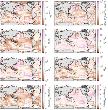
coefficient [Janssen, 2000]. Salinity is taken from the 2009 World Ocean Atlas [Antonov et al., 2010]. The ratio between the sourcefluxes from (3) and (4) andNorris et al. [2012] is shown in Figure 3 forR80= 0.5μm. Also shown arefields of
U10, theNorris et al. [2012] sourceflux,RHa,RHw,Hs, and
the ratioHs/Hfd where Hfd is the value ofHs for waves in
equilibrium with the local wind, calculated from the WAM model wind-wave relation [Wave Model Development and Implementation Group, 1988]; Hs/Hfd gives a measure of
[image:4.612.122.495.57.439.2]the degree of wave development. In order to avoid any bias that might result from extrapolating the source functions
Figure 3. Global distributions of (a) wind speed, U10; (b) SSAflux fromNorris et al. [2012]; (c) significant wave height,Hs;
(d)Hs/Hfd; (e)RHa; (f)RHw; (g) ratio of sea spray sourceflux dF/dR80from theRHa(3) and U10[Norris et al., 2012]
param-eterizations atR80= 0.5μm; and (h) same as Figure 3g but forRHw. Example regions where the Reynolds number function is
beyond the range of conditions from which they were derived, we have excluded grid points with winds outside the observed range of 4<U10<18 m s1.
[12] There are some substantial differences between the
parameterizations; the RHa parameterization ranges from
less than 0.1 of the U10 source function to about 3 times
larger; the RHwfunction peaks at 5 times larger. A
compar-ison of the spatial distribution of the differences to those of the forcing parameters is revealing. Considerfirst theRHa
function (Figure 3g). The regions where its ratio with the U10function is largest coincide not with the highest winds
or Reynolds numbers in storm systems, but around the margins of these systems. These are regions where the wavefield is significantly better developed than the equilib-rium wavefield for the local wind (Hs/Hfd>1); two such
regions are indicated by purple boxes. In regions where the wave state is underdeveloped compared to the equilib-rium state—notably in the regions of highest wind speed within storm systems—theRHaparameterization falls below
the U10 parameterization; examples are indicated by the
brown boxes. The RHw parameterization follows a similar
spatial pattern but predicts somewhat higher fluxes over the tropical and subtropical oceans. This is a consequence of the stronger temperature dependence of water viscosity compared to that of air. The implications of this and the lim-itations it imposes on the interpretation of our results are discussed below.
4. Conclusions
[13] New parameterizations of the sea spray source flux
(0.176<R80<6.61μm) have been derived as functions of
wave Reynolds numbers, RHa and RHw. They account for
up to twice the variance in the measured fluxes than does wind speed alone. The variance explained decreases with particle size for all three parameterizations; at the smallest sizes, U10 and RH account for similar variance, and that
explained by U10 then falls more rapidly with particle size
than that for RHa and RHw. The size dependence of R2 is
consistent with Norris et al. [2013] who found that SSA production per unit area whitecap was wind speed depen-dent for R80<2μm, but showed no clear relationship at
larger sizes. We speculate that this behavior is related to changes in bubble populations with increasing wind and wave breaking—Norris et al. [2013] found that concentra-tions of small bubbles increased more than those of large bubbles with increasing wind speed—and the sizes of aero-sol particles generated by different-sized bubbles. Here, jet drops will dominate production for R80>1μm and film
drops forR80<1μm.
[14] A comparison of the ratio of the new
parameteriza-tions to the wind speed-dependent function derived by
Norris et al. [2012] from the same data set shows differ-ences of a factor of 0.1 to 3 (RHa) and 5 (RHw). Fluxes higher
than those of the U10function are found around the margins
of storm systems where propagation of waves away from the regions of highest winds results in wave states that are overdeveloped compared to the equilibrium state for the local wind. Fluxes lower than those from the U10function
are found where the wave state is underdeveloped. We emphasize that both the U10 and RH-dependent source
functions are derived from the same in situ measurements; differences between them arise almost entirely from the
inclusion of information on wave state via the Reynolds number. Superficially, the results appear contrary to those of
Norris et al. [2012] that theflux was higher in undeveloped seas for a given wind speed. In fact, there is no direct contra-diction.Norris et al. [2012] characterized wave development by the mean wave slope; this depends only onHsand Tz, the
zero-crossing period of the waves, and says nothing about the relationship between the observed waves and those expected under equilibrium with the local wind.
[15] TheRHwfunction predicts largerfluxes thanRHaover
much of the ocean—a result of the stronger temperature dependence of viscosity for water than for air. The observa-tions used to derive the source funcobserva-tions span a limited range of temperatures. This leaves open the possibility that viscos-ity-dependent properties of wave breaking or bubbles might affect the SSAflux in a manner not accounted for by these source functions. Measurements under a much wider range of conditions are required to address this issue. The data set is also not large enough to assess any separate impact of wind waves and swell, nor of relative wind and wave directions, both of which may complicate the wind-wave-flux relation-ship [e.g.,Goddijn-Murphy et al., 2011]. Thus, the source functions proposed cannot be considered universal but are a significant step toward this goal and an improvement on sim-ple wind speed-dependent functions.
[16] At any given time, the wave state over the majority of
the world’s oceans is out of equilibrium with the local wind
—the majority being overdeveloped and dominated by swell; just 8.5% is found to be underdeveloped in the ECMWFfields by the Wave Model Development and Implementation defi ni-tion. Simple wind speed-dependent SSA source functions will tend to misrepresent the spatial variability of SSA production. This has implications for modeling of new particle formation and regional aerosol budgets, marine atmospheric boundary layer chemistry, and the spatial variability of cloud condensa-tion nuclei concentracondensa-tions over the oceans. The new parame-terizations are readily implemented in models and should lead to better representation of the spatial and temporal vari-ability of sea sprayfluxes.
[17] Acknowledgments. This work was funded by the UK Natural Environment Research Council grants NE/C001842/1 as part of UK SOLAS, NE/G00353X/1, and NE/G000107/1. We thank the Captain and crew of the RRSDiscoveryand the staff of National Marine Facilities Sea Systems for their assistance in preparing for and during the cruise, ECMWF for the global model reanalysisfields, and David Woolf and an anonymous reviewer for their constructive comments on the manuscript.
[18] The Editor thanks David Woolf and an anonymous reviewer for their assistance in evaluating this paper.
References
Andreae, M. O., and D. Rosenfeld (2008), Aerosol-cloud-precipitation inter-actions, Part 1. The nature and sources of cloud-active aerosols,Earth-Sci. Rev.,89, 13–41, doi:10.1016/j.earscirev.2008.03.001.
Anguelova, M. D., and F. Webster (2006), Whitecap coverage from satellite measurements: Afirst step toward modeling the variability of oceanic whitecaps,J. Geophys. Res.,111, C03017, doi:10.1029/2005JC003158. Antonov, J. I., D. Seidov, T. P. Boyer, R. A. Locarnini, A. V. Mishonov,
H. E. Garcia, O. K. Baranova, M. M. Zweng, and D. R. Johnson (2010), inWorld Ocean Atlas 2009, Volume 2: Salinity, edited by S. Levitus, 184 pp., NOAA Atlas NESDIS 69, U.S. Government Printing Office, Washington, D.C.
Brooks, I. M., et al. (2009a), Physical exchanges at the air-sea interface: Field measurements from UK-SOLAS,Bull. Am. Meteorol. Soc., 90, 629–644, doi:10.1175/2008BAMS2578.1.
Brooks, I. M., et al. (2009b), UK-SOLASfield measurements of air-sea exchange: Instrumentation,Bull. Am. Meteorol. Soc.,90, (electronic sup-plement), 9–16, doi:10.1175/2008BAMS2578.2.
de Leeuw, G., E. L. Andreas, M. D. Anguelova, C. W. Fairall, E. R. Lewis, C. O’Dowd, M. Schulz, and S. E. Schwartz (2011), Productionflux of sea-spray aerosol,Rev. Geophys.,49, RG2001, doi:10.1029/2010RG000349. Goddijn-Murphy, L., D. K. Woolf, and A. H. Callaghan (2011), Parameterizations and algorithms for oceanic whitecap coverage,J. Phys. Oceanogr.,41, 742–756, doi:10.1175/2010JPO4533.1.
Hill, M. K., B. J. Brooks, S. J. Norris, M. H. Smith, I. M. Brooks, G. de Leeuw, and J. J. N. Lingard (2008), A Compact Lightweight Aerosol Spectrometer Probe (CLASP),J. Atmos. Oceanic Technol.,25, 1996–2006, doi:10.1175/2008JTECHA1051.1.
Hoppel, W. A., G. M. Frick, and J. W. Fitzgerald (2002), The surface source function for sea-salt aerosol and aerosol dry deposition to the ocean sur-face,J. Geophys. Res.,107(D19), 4382, doi:10.1029/2001JD002014. Intergovernmental Panel on Climate Change (2007), Climate Change
2007: The Physical Science Basis: Working Group I Contribution to the Fourth Assessment Report of the Intergovernmental Panel on Climate Change, edited by S. Solomon et al., 996 pp., Cambridge Univ. Press, New York.
Janssen, P. A. E. M. (2000), ECMWF wave modeling and satellite altimeter wave data, inSatellites, Oceanography and Society, edited by D. Halpern, pp. 35–56, Elsevier, Amsterdam.
Lewis, E. R., and S. E. Schwartz (2004),Sea Salt Aerosol Production: Mechanisms, Methods, Measurements, and Models—A Critical Review, Geophys. Monogr. Ser., vol.152, 413 pp., AGU, Washington, D. C. Liu, B., C. L. Guan, L. A. Xie, and D. L. Zhao (2012), An investigation of the
effects of wave state and sea spray on an idealized typhoon using an air–sea coupled modelling system,Adv. Atmos. Sci.,29, 391–406, doi:10.1007/ s00376-011-1059-7.
Mårtensson, E. M., E. D. Nilsson, G. de Leeuw, L. H. Cohen, and H. C. Hansson (2003), Laboratory simulations and parameterization of the primary marine aerosol production, J. Geophys. Res., 108(D9), 4297, doi:10.1029/2002JD002263.
Merikanto, J., D. V. Spracklen, G. W. Mann, S. J. Pickering, and K. S. Carslaw (2009), Impact of nucleation on global CCN,Atmos. Chem. Phys.,9, 8601–8616, doi:10.5194/acp-9-8601-2009.
Monahan, E. C. (1986), The ocean as a source for atmospheric particles, in
The Role of Air-Sea Exchange in Geochemical Cycling, Buat-Menard, edited by D. Reidel, 129–163 pp., Publishing Company, Dordrecht. Monahan, E., and I. O’Muircheartaigh (1980), Optimal power-law
descrip-tion of oceanic whitecap coverage dependence on wind speed,J. Phys. Oceanogr.,10, 2094–2099.
Monahan, E. C., D. E. Spiel, and K. L. Davidson (1986), A model of marine aerosol generation via whitecaps and wave disruption, in Oceanic
Whitecaps, edited by E. C. Monahan and G. Mac Niocaill, pp. 167–174, D. Reidel Publishing Company, Dordrecht.
Montgomery, R. B. (1947), Viscosity and thermal conductivity of air and diffusivity of water vapor in air,J. Meteorol.,4, 193–196.
Norris, S. J., I. M. Brooks, M. K. Hill, B. J. Brooks, M. H. Smith, and D. A. J. Sproson (2012), Eddy covariance measurements of the sea spray aerosol flux over the open ocean, J. Geophys. Res., 117, D07210, doi:10.1029/2011JD016549.
Norris, S. J., I. M. Brooks, B. I. Moat, M. J. Yelland, G. de Leeuw, R. W. Pascal, and B. J. Brooks (2013), Field measurements of aerosol pro-duction from whitecaps in the open ocean, Ocean Sci., 9, 133–145, doi:10.5194/os-9-133-2013.
Sharqawy, M. H., J. H. Lienhard, and S. M. Zubair (2010), Thermophysical properties of seawater: A review of existing correlations and data,Desalin. Water Treat.,16, 354–380, doi:10.5004/dwt.2010.1079.
Shi, J., D. Zhao, X. Li, and Z. Zhong (2009), New wave-dependent formulae for sea sprayflux at air-sea interface,J. Hydrodyn.,21, 573–581. Smith, M. H., P. M. Park, and I. E. Consterdine (1993), Marine aerosol
con-centrations and estimatedfluxes over the ocean,Q. J. R. Meteorol. Soc.,
119, 809–824, doi:10.1002/qj.49711951211.
Sproson, D. A. J., I. M. Brooks, and S. J. Norris (2013), The effect of hygroscop-icity on sea spray aerosolfluxes: A comparison of high-rate and bulk correc-tion methods,Atmos. Meas. Tech.,6, 323–335, doi:10.5194/amt-6-323-2013. Toba, Y., and M. Koga (1986), A parameter describing overall conditions of wave breaking, whitecapping, sea-spray production and wind stress, in
Oceanic Whitecaps, edited by E. C. Monahan and G. Mac Niocaill, pp. 37–47, Springer, New York.
Tucker, M. J., and E. G. Pitt (2001),Waves in Ocean Engineering, Ocean Eng. Book Ser., vol.5, 521 pp., Elsevier, New York.
Wave Model Development and Implementation Group (1988), The WAM model: A third generation ocean wave prediction model, J. Phys. Oceanogr.,18, 1775–1810.
Woolf, D. K. (2005), Parametrization of gas transfer velocities and sea-state-dependent wave breaking,Tellus,57A, 87–94.
Zábori, J., R. Krejci, A. M. L. Ekman, E. M. Mårtensson, J. Ström, G. de Leeuw, and E. D. Nilsson (2012), Wintertime Arctic Ocean sea water properties and primary marine aerosol concentrations, Atmos. Chem. Chem. Phys.,12, 0405–10421, doi:10.5194/acp-12-10405-2012. Zhao, D., and Y. Toba (2001), Dependence of whitecap coverage on wind
and wind-wave properties,J. Oceanogr.,57, 603–616.