On the acceleration of wavefront applications using distributed many-core architectures

This is a repository copy of

On the acceleration of wavefront applications using distributed

many-core architectures

.

White Rose Research Online URL for this paper:

http://eprints.whiterose.ac.uk/136612/

Version: Accepted Version

Article:

Pennycook, S. J., Hammond, S. D., Mudalige, G. R. et al. (2 more authors) (2012) On the

acceleration of wavefront applications using distributed many-core architectures.

Computer Journal. pp. 138-153. ISSN 0010-4620

https://doi.org/10.1093/comjnl/bxr073

[email protected] https://eprints.whiterose.ac.uk/ Reuse

Items deposited in White Rose Research Online are protected by copyright, with all rights reserved unless indicated otherwise. They may be downloaded and/or printed for private study, or other acts as permitted by national copyright laws. The publisher or other rights holders may allow further reproduction and re-use of the full text version. This is indicated by the licence information on the White Rose Research Online record for the item.

Takedown

If you consider content in White Rose Research Online to be in breach of UK law, please notify us by

On the Acceleration of Wavefront Applications

using Distributed Many-Core Architectures

S.J. Pennycook∗1

, S.D. Hammond∗, G.R. Mudalige†, S.A. Wright∗, S. A. Jarvis∗

∗_{Performance Computing and Visualisation}

Department of Computer Science University of Warwick, UK

†_{Oxford eResearch Centre}

University of Oxford Oxford, UK

Abstract—In this paper we investigate the use of distributed GPU-based architectures to accelerate pipelined wavefront ap-plications – a ubiquitous class of parallel algorithm used for the solution of a number of scientific and engineering applications. Specifically, we employ a recently developed port of the LU solver (from the NAS Parallel Benchmark suite) to investigate the performance of these algorithms on high-performance computing solutions from NVIDIA (Tesla C1060 and C2050) as well as on traditional clusters (AMD/InfiniBand and IBM BlueGene/P). Benchmark results are presented for problem classes A to C and a recently developed performance model is used to provide projections for problem classes D and E, the latter of which represents a billion-cell problem. Our results demonstrate that while the theoretical performance of GPU solutions will far exceed those of many traditional technologies, the sustained application performance is currently comparable for scientific wavefront applications. Finally, a breakdown of the GPU solu-tion is conducted, exposing PCIe overheads and decomposisolu-tion constraints. A new k-blocking strategy is proposed to improve the future performance of this class of algorithm on GPU-based architectures.

Index Terms—Wavefront; GPU; Many-Core Computing; CUDA; Optimisation; Performance Modelling

I. INTRODUCTION

The fundamental design of high performance supercom-puters is on the verge of a significant change. The arrival of petascale computing in 2008, with the IBM RoadRunner supercomputer, represented a departure from the large-scale use of commodity processors to hybrid designs employing heterogeneous computational accelerators. Although the pre-cise design of RoadRunner remains unique, the utilisation of computational “accelerators” such as field programmable gate arrays (FPGAs), graphics processing units (GPUs) and the forthcoming Knights-range of “many-integrated core” (MIC) products from Intel has gained significant interest throughout the high performance computing (HPC) community. These designs show particular promise because of the high levels of spatial and power efficiency which can be achieved in comparison to general-purpose processors – both of which represent significant concerns in the design of petascale and exascale supercomputers in the coming decade.

1_{Email:[email protected]}

However, despite the impressive theoretical peak perfor-mance of accelerator designs, several hardware/software devel-opment challenges must be met before high levels ofsustained

performance can be achieved by HPC codes on these architec-tures. First, an increase in available cores/threads has lead to a decrease in the amount of memory per processing element. This means that algorithms constructed under the assumption of high-powered processors with large memories may not port well to these new platforms; typically their parallel efficiency when run at scale on accelerator-based clusters is very poor. Second, there has been a trend in many early publications on the subject of accelerator-based designs to compare general-purpose CPUs in unfair terms. This has given an impression that large performance gains are achievable for most HPC codes.

The effect is that code custodians are faced with difficult choices when considering future architectures and future code developments. It is therefore important that the community develop an understanding of (i) which classes of application; (ii) which methods of code porting; and (iii) which code optimisations/designs are likely to lead to notable performance gains when accelerators are employed.

It is to this end that we investigate, through implementation, benchmarking and modelling, the performance of pipelined

wavefront applicationson devices employing NVIDIA’s

for how a fullcode will perform.

The contributions of this paper are as follows:

• We present a study of porting and optimising the LU

benchmark for the CUDA GPU architecture. The study includes code optimisations and the selection of advanced compiler options for improved CPU and GPU perfor-mance;

• The GPU-accelerated solution is benchmarked on a

selec-tion of GPUs, ranging from workstaselec-tion-grade commod-ity GPUs to NVIDIA’s HPC products. This study2 is the first known work to feature an independent performance comparison of the Tesla C1060 and C2050 for a pipelined wavefront application. The results include comparative benchmarking results from Nehalem-class CPUs, so that we can contrast the CPU and GPU solutions for LU Class A-C problems;

• Two recently developed application performance

mod-els (one analytical [2] and one based on discrete-event simulation [3]) are used to project the benchmark re-sults to systems (and problems) of larger scale. Us-ing two modellUs-ing techniques gives us greater confi-dence in our results as we compare GPU-based clusters against two alternative designs – a socket, quad-core AMD Opteron/InfiniBand-based cluster and an IBM BlueGene/P. Projections are provided for strong-scaled Class D and E problems, as well as for LU in weak-scaled configurations. The results provide insight into how the performance of this class of code will scale on petascale-capable architectures;

• The performance models are used to deconstruct the

execution costs of the GPU solution, allowing us to examine the proportions of runtime accounted for by communication between nodes, as well as over the PCI-Express (PCIe) bus. Using this information we propose a new k-blocking strategy for LU to improve the future performance of this class of algorithm on GPU-based architectures.

The remainder of this paper is organised as follows: Section II discusses previous work, and Section III describes the operation of the LU benchmark and the CUDA programming model; in Section IV we detail the CUDA implementation of the LU benchmark and Section V outlines the optimisations applied to both the CPU and GPU versions of the code; Section VI presents a performance comparison of the CPU and GPU codes running on single workstations, including several NVIDIA GPUs of different compute capability; Section VII discusses the performance models used in this work and validates them against benchmark data; Section VIII presents both weak- and strong-scaling studies of the CPU and GPU implementations of the benchmark; Section IX discusses the issues affecting the scalability of the GPU implementation and presents a newk-blocking strategy for this class of algorithm; Section X concludes the work and discusses future research.

2_{including the original workshop paper that this paper extends}

II. RELATEDWORK

We present a port of the LU benchmark to NVIDIA’s CUDA architecture. LU belongs to a class of applications known

as pipelined wavefront computations, which are characterised

by their parallel computation and communication pattern. The performance of such applications is well understood for conventional multi-core-processor-based clusters [2], [4] and a number of studies have investigated the use of accelerator-based architectures for the Smith-Waterman string matching algorithm (a two-dimensional wavefront algorithm) [5], [6], [7]. However, performance studies for GPU-based implemen-tations of three-dimensional wavefront applications (either on a single device or at cluster scale) remain scarce; to our knowledge, our implementation of LU is the first such port of this specific code to a GPU.

Two previous studies [8], [9] detail the implementa-tion of a different three-dimensional wavefront applicaimplementa-tion, Sweep3D [10], on accelerator-based architectures. The first of these [8] utilises the Cell Broadband Engine (B.E.), exploiting five levels of parallelism in the implementation. The perfor-mance benefits of each are shown in order, demonstrating a clear path for the porting of similar codes to the Cell B.E. architecture. In the second [9], the Sweep3D benchmark is ported to CUDA and executed on a single Tesla T10 processor. Four stages of optimisation are presented: the introduction of GPU threads, using more threads with repeated computation, using shared memory and using a number of other methods that contribute only marginally to performance. The authors conclude that the performance of their GPU solution is good, extrapolating from speedup figures that it is almost as fast as the Cell B.E. implementation described in [8].

These studies suggest that accelerator-based architectures are a viable alternative to traditional CPUs for pipelined wavefront codes. However, one must be cautious when reading speedup figures: in some studies the comparison between execution times is made between an optimised GPU code and an un-optimised CPU code [11]; in other work we do not see the overhead of transferring data across the PCIe bus [12]; in some cases the CPU implementation is serial [13]; in others, parallel CPU and GPU solutions are run at different scales [14], or the CPU implementation is run on outdated hardware [9]. This is not the first paper to dispute such speedup figures [15], [16] and others have highlighted the importance of hand-tuning CPU code when aiming for a fair comparison [17], [18].

This paper is an extension of the work originally presented in [19], which itself appeared as a Feature Article inHPC Wire

in November 2010 [20]. This extended paper: (i) documents additional optimisations to both the CPU and GPU codes – in comparison to the results in [19], the benchmarked times reported here are up to 26.9% faster and are thus more representative of the raw performance of each architecture; (ii) extends the performance modelling to include additional weak-scaling results (to complement the strong-scaling results previously presented); (iii) decomposes the runtime costs to expose the impact of communication between nodes and over the PCIe bus; and (iv) proposes a new k-blocking strategy for LU, to improve the future performance of this class of algorithm on GPU-based architectures.

III. THELU BENCHMARK

The LU benchmark belongs to the NAS Parallel Bench-mark (NPB) suite, a set of parallel aerodynamic simulation benchmarks. The code implements a simplified compressible Navier-Stokes equation solver, which employs a Gauss-Seidel relaxation scheme with symmetric successive over-relaxation (SSOR) for solving linear and discretised equations. The reader is referred to [1] for a thorough discussion of the mathematics. In brief, the code solves the (n+ 1)th

time step of the discretised linear system:

Un+1_=Un_{+ ∆U}n using:

Kn_∆Un_=Rn

whereKis a sparse matrix of sizeNx⇥Ny⇥Nzand each of its matrix elements is a 5⇥5 sub-matrix. An SSOR-scheme is used to expedite convergence with the use of an over-relaxation factorδ2(0,2), such that:

Un+1

=Un_{+ (1/(δ(2−δ))∆U}n

The SSOR operation is re-arranged to enable the calculation to proceed via the solution of a regular sparse, block-lower (L) and upper (U) triangular system (giving rise to the name LU). The algorithm proceeds through the computing of the right-hand-side vector Rn

, followed by the computing of the lower-triangular and then upper-triangular solutions. Finally the solution is updated.

In practice, the three-dimensional data grid used by LU is of size N3

(i.e. the problem is always a cube), although the underlying wavefront algorithm works equally well on grids of all sizes. As of release 3.3.1, NASA provide seven different application “classes” for which the benchmark is capable of performing verification: Class S (123_{), Class W (33}3

), Class A (643_{), Class B (102}3_{), Class C (162}3_{), Class D (408}3

) and Class E (10203

). GPU performance results for Classes A through C are presented in Section VI; due to the lengthy execution times and significant resource demands associated with Classes D and E, benchmarked times and projections are

shown for cluster architectures in Section VIII. The use of these standard problem classes in this work ensures that our results are directly comparable to those reported elsewhere in the literature.

In the MPI implementation of the benchmark, this data grid is decomposed over a two-dimensional processor array of size

Px⇥Py, assigning each of the processors a stack of Nz data “tiles” of size Nx/Px⇥Ny/Py⇥1. Initially, the algorithm selects a processor at a given vertex of the processor array which solves the first tile in its stack. Once complete, the edge data (which has been updated during this solve step) is communicated to two of its neighbouring processors. These adjacent processors – previously held in an idle state via the use of MPI-blocking primitives – then proceed to compute the first tile in their stacks, while the original processor solves its second tile. Once the neighbouring processors have completed their tiles, their edge data is sent downstream. This process continues until the processor at the opposite vertex to the starting processor solves its last tile, resulting in a “sweep” of computation through the data array.

Such sweeps, which are the defining features of pipelined wavefront applications, are also commonly employed in parti-cle transport codes such as Chimaera [2] and Sweep3D [10]. This class of algorithm is therefore of commercial as well as academic interest, not only due to its ubiquity, but also the significant time associated with its execution at large supercomputing sites such as NASA, the Los Alamos National Laboratory (LANL) in the US and the Atomic Weapons Establishment (AWE) in the UK.

LU is simpler in operation than Sweep3D and Chimaera in that it only executes two sweeps through the data grid (as opposed to eight), one from the vertex at processor 0, and another in the opposite direction. The execution time for a single instance of LU itself is not very significant, taking in the order of minutes. Nonetheless, it provides an oppor-tunity to study a representative science benchmark which, when scaled or included as part of a larger work flow, can consume vast amounts of processing time. The principle use of the LU benchmark is comparing the suitability of different architectures for production CFD applications [21] and thus the results presented in this paper have implications for large-scale production codes. LU’s memory requirements are also significant (approximately 160GB for a Class E problem), necessitating the use of large machines.

The pseudocode in Algorithm 1 details the SSOR loop that accounts for the majority of LU’s execution time.

Algorithm 1 Pseudocode for the SSOR loop.

foriter= 1_{tomax iter do}

fork= 1_toNz do calljacld(k)

callblts(k)

end for

fork=_Nz to1do calljacu(k)

callbuts(k)

end for

calll2norm()

callrhs()

calll2norm()

end for

compile- and run-time, but is typically 250 - 300 in Classes A through E.

A. CUDA Architecture/Programming Model

Our GPU implementation makes use of NVIDIA’s CUDA programming model, since it is presently the most mature and stable model available for the development of GPU computing applications. We provide a brief overview of the CUDA architecture/programming model; for an in-depth description the reader is directed to [22].

A CUDA-capable NVIDIA GPU is an example of a many-core architecture, composed of a large quantity of relatively low-powered cores. Each of the GPU’sstream multiprocessors

(SMs) consist of a number of stream processors (SPs) that share control logic and an instruction cache. All communi-cation between the CPU (or host) and the GPU (or device) must be carried out across a PCIe bus. The exact hardware specification of a CUDA GPU depends upon its range and model; the number of SPs, the amount of global (DRAM) and shared memory and so-called “compute capability” all vary by card. Specifications of the GPUs used in our study are listed in Table I.

Each minor revision to compute capability represents the addition of new features, whilst each major revision represents a change to the core architecture (e.g.the move from Tesla to Fermi represents a move from 1.0 to 2.0). Support for double-precision floating-point arithmetic was not introduced until revision 1.2.

Functions designed for the GPU architecture are known as

kernelsand, when launched, are executed simultaneously in a

multiple-data (SIMD) or single-instruction-multiple-thread (SIMT) fashion on a large number of threads. These threads are lightweight – with program kernels typically being launched in configurations of up to thousands of threads

a_{2.65GB with ECC-enabled.}

b_{48kB is available if the programmer selects for higher shared memory}

instead of larger L1 cache.

GeForce Tesla 8400GS 9800GT C1060 C2050

Cores 8 112 240 448

Clock _{1.40GHz 1.38GHz 1.30GHz 1.15GHz} Rate

Global

0.25GB 1GB 4GB 3GBa Memory

Shared

16kB 16kB 16kB 16kBb

Memory

Compute _{1.1 1.1 1.3 2.0} Cap.

TABLE I

CUDA GPUSPECIFICATIONS.

– and are arranged into one-, two- or three-dimensionalblocks, with blocks forming a one- or two-dimensional grid. This programming model allows developers to exploit parallelism at two levels – the thread-blocks are assigned to SMs and executed in parallel, whilst the SPs (making up an SM) execute the threads of a thread-block in groups of 32 known aswarps. In order to permit CUDA programs to scale up or down to fit different hardware configurations, these thread blocks can be scheduled for execution in any order. However, this scalability is not without cost; unless carefully designed, programs featuring global thread synchronisation are likely to cause deadlocks. Indeed, the CUDA programming model does not provide any method of global thread synchronisation within kernels for this reason. There is, however, an implicit global thread synchronisation barrier between separate kernel calls.

IV. GPU IMPLEMENTATION

Version 3.2 of the LU benchmark, on which our work is based, is written in FORTRAN 77 and utilises MPI for communica-tion between processing-elements. The GPU implementacommunica-tion makes use of NVIDIA’s CUDA. The standard language choice for developing CUDA programs is C/C++ and, although the Portland Group offer a commercial alternative allowing the use of CUDA statements within FORTRAN 77 applications, the first stage in our porting of LU was to convert the entire application to C.

To provide a comparison of the performance trade-offs for CFD codes in using single- or double-precision floating-point arithmetic, the ported version of the benchmark was instru-mented to allow the selection of floating-point type at compile time. Although NASA explicitly requests the use of double-precision in the benchmark suite, we have included single-precision calculations to allow us to measure the performance of consumer GPU devices. The accuracy of these single-precision solutions is lower (i.ethe error exceeds the default epsilon of 10−8

0 100 200 300 400 500 600

A B C

Ex

ecution

T

ime

(Seconds)

Problem Class C SP

C (SMT) SP FORTRAN 77 SP FORTRAN 77 (SMT) SP C DP C (SMT) DP FORTRAN 77 DP FORTRAN 77 (SMT) DP

Fig. 1. Execution times for FORTRAN 77 and C implementations of LU.

For all single-precision executions described in this paper a manual check of the resulting output was performed to ensure that the solution was comparable to its double-precision equivalent.

Figure 1 shows a performance comparison of the original FORTRAN 77 code with our C port, running on an Intel X5550 in both single (SP) and double (DP) precision. The execution times given for the C port are prior to the use of a GPU (i.e. all mathematics are ported and running on only the CPU). As shown by the graph, the original FORTRAN 77 implementation is approximately 1.4x faster than our C port running on identical hardware.

There are two differences between the C and FORTRAN 77 implementations that are likely to be the cause of this perfor-mance gap: firstly, the port to C was structured from the outset to be more amenable to CUDA, rather than being optimised for CPU execution; and secondly, the multi-dimensional solution arrays are statically allocated in the FORTRAN 77 code, but dynamically allocated in the C code. The fact that the C code is slower demonstrates that the performance improvements shown in Sections VI and VIII come from the utilisation of the GPU, rather than from any optimisations introduced during the process of changing programming language.

At the time of writing, the maximum amount of memory available on a single CUDA GPU is 6GB (available in the Tesla C2070). At least 10GB is required to solve a Class D problem, thus the use of MPI is necessary if the code is to be able to solve larger problems than Class C. Our CUDA implementation retains and extends the MPI-level parallelism present in the original benchmark, mapping each of the MPI tasks in the system to a single CPU core, which is in turn responsible for controlling a single GPU.

The parallel computation pattern of wavefront applications involves a very strict dependency between grid-points. Lam-port’s original description of the Hyperplane algorithm in [23] demonstrated that the values of all grid-points on a given

hyperplane defined by i+j +k = f can be computed in

parallel, with the parallel implementation looping overfrather

0 2

1 0

!

2 2

5

7

0

5

6

3 4

1

Fig. 2. Two-dimensional mapping of threads in a thread-block onto the entire three-dimensional grid.

than i, j and k. In order to ensure that the dependency is satisfied, it is necessary that we have a global synchronisation barrier between the solution of each hyperplane; since the CUDA programming model does not support global synchro-nisation withinkernels, each hyperplane must be solved by a separate kernel launch. As shown in Figure 2, which details the mapping of threads to grid-points on a hyperplane, the first kernel is responsible for computing the value of one grid-point, the second for three, the third for six and so on.

V. OPTIMISATION

A. Loop Unrolling and Fusion

Each of the solution arrays in LU is a four-dimensional array of the form(k, j, i, m), wheremranges from 0 to 4 and

i,j andkrange from 0 to(Nx−1),(Ny−1)and(Nz−1) respectively. In the vast majority of the loop nests encountered in blts, buts, rhs and l2norm, the inner-most loop is over these five values ofm.

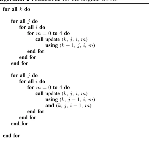
Algorithm 2 Pseudocode for the originalblts.

for allkdo

for allj do for allido

form= 0 to4do callupdate (k,j,i,m)

using(k−1,j,i,m)

end for end for end for

for allj do for allido

form= 0 _to4_do callupdate (k,j,i,m)

using(k,j−1,i,m)

and(k, j,i−1,m)

end for end for end for

end for

both CPUs and GPUs (but at the expense of increased register pressure).

We also fuse the two sets of loops overj andiinto a single set of loops, mainly for the benefit of the GPU implementation: it enables a single kernel to carry out the updates in all three neighbouring directions, as opposed to requiring a separate kernel for each of the loops overjandi; it enables the GPU to hide memory latency much more effectively, as fewer memory loads need to be completed before the solution can be updated in the j and i directions; the number of registers required to hold intermediate values is decreased, which may increase occupancy (i.e. the ratio of active warps to the maximum number of warps supported on a single SM).

Pseudocode for our optimised implementation of blts is shown in Algorithm 3.

Algorithm 3 Pseudocode for the optimisedblts.

for allkdo for alljdo

for allido

callupdate (k,j,i,0)

using(k−1,j,i,0)

.. .

callupdate (k,j,i,4₎ using(k−1,j,i,4)

callupdate (k,j,i,0₎ using(k,j−1,i,0)

.. .

callupdate (k,j,i,4₎ using(k,j−1,i,4)

callupdate (k,j,i,0₎ using(k,j,i−1,0)

.. .

callupdate (k,j,i,4₎ using(k,j,i−1,4)

end for end for end for

B. Memory Access Optimisation

For each grid-point, thejacldandjacumethods read in five solution values and five values from three neighbours (20 values in total). These data are used to populate four 5⇥5 matrices (100 values in total) per grid-point, which are later used by thebltsandbutsmethods. In our optimised code, we move this calculation into the wavefront section; instead of loading 100 values per grid-point, we load 20 values and perform thejacldandjacucalculations inline.

In addition to reducing the amount of memory required for each problem size, this optimisation decreases the number of memory accesses made by the blts and buts kernels, whilst increasing their computational intensity. This improves

Processor 0

kblock

Processor 1 Processor 2

Fig. 3. Thek_{-blocking policy.}

the GPU’s ability to hide the latency of the remaining memory accesses.

Recent work [24], which investigates a space/time tradeoff in GPU codes, reaches a similar conclusion – that it is beneficial to compress data structures in order to decrease the frequency and size of memory accesses at the expense of more floating-point arithmetic operations.

C. Message Size Optimisation

The majority of the messages sent by LU are small, since each processor works on a single tile of data (of sizeNx/Px⇥

Ny/Py⇥1) at a time. Each of the messages sent during the wavefront section contains a single row or column of either

Nx/PxorNy/Py floating-point values, which does not make efficient use of network bandwidth.

To address this, we implement a system we refer to hence-forth as k-blocking, which is implemented in the Sweep3D benchmark. Under this system, as shown by Figure 3, each processor computes the values of a stack of kblock tiles prior to communicating with its neighbouring processors. Each message now consists of a face ofNx/Px⇥kblock or

Ny/Py⇥kblockfloating-point values and adjusting the value of kblock allows us to achieve better network (and/or PCIe bus) efficiency. In the GPU solution,k-blocking also increases the amount of available parallelism; rather than carrying out a two-dimensional wavefront sweep across each tile, we can carry out a three-dimensional wavefront sweep across the stack of kblocktiles.

The optimal value of thiskblockparameter differs according to architecture, and also whether we are operating on a single processor or a collection of processors communicating via MPI. On a single processor, the best value of kblock is Nz, since it maximises the size of the hyperplanes that can be processed in each parallel step.

choosing too large a kblockwill cause delays to downstream processors. For GPUs, the amount of parallelism is another important factor: too small a kblock will limit the amount of available parallelism, but too large a kblock will again cause pipeline delays. Due to this tradeoff, it is necessary to choose an optimal value ofkblockvia empirical evaluation or performance modelling.

On the CPU, we typically set kblock = 1, as the negative effect of larger values on pipeline fill time tends to outweigh the positive effects upon bandwidth efficiency. In theory, the selected kblock value for the GPU should be greater than or equal to Nx/Px +Ny/Py −1, since this is the number of wavefront steps required to complete a single tile and (generally) to reach the largest hyperplane. In practice however, we find that the increase in parallel efficiency is outweighed by the increase in pipeline fill time; we instead set kblock=min(Nx/Px, Ny/Py), as this strikes a balance between the reduction in parallelism and increase in pipeline fill time. Empirical benchmarking confirms that these values of kblock provide the best levels of performance. Although we do not use auto-tuning, this approach could also be used to establish parameter settings that maximise per-machine performance.

D. GPU-specific Optimisation

We ensure that each of our memory accesses iscoalesced, in keeping with the guidelines in [22]. The simplest way to achieve this is to ensure that all threads access contiguous memory locations; for the wavefront sections, we rearrange memory in keeping with the thread allocation depicted in Figure 2.

However, the parallel sections with no data dependencies require a different memory arrangement and therefore be-tween the two sections we call a rearrangement kernel to swap memory layouts. Although this kernel involves some uncoalesced memory accesses, which is largely unavoidable since it reads from one memory layout and writes to another, the penalty is incurred only once – rather than for every memory access within the methods themselves. The lack of global synchronisation within CUDA kernels prevents this rearrangement from being performed in place and therefore we make use of a separate rearrangement buffer on the GPU. Though this does increase the memory requirement of the GPU solution, the size of the rearrangement buffer is significantly less than the combined size of the arrays removed as part of the optimisation detailed in Subsection V-B.

Since the CUDA card itself does not have access to the network, any data to be sent via MPI must first be transferred to the CPU and, similarly, any data received via MPI must be transferred to the GPU. Packing or unpacking the MPI buffers on the CPU requires a copy of the entire data grid – carrying out this step on the GPU significantly decreases the amount of data sent across the PCIe bus and also allows for the elements of the MPI buffers to be packed or unpacked in parallel.

Device Compiler Options

Intel X5550 (Fortran)

Sun Studio 12 (Update 1)

-O5 -native -xprefetch -xunroll=8 -xipo -xvector

Intel X5550

(GPU Host) GNU 4.3

-O2 -msse3 -funroll-loops

GeForce

8400GS/9800GT NVCC -O2 -arch="sm_11"

Tesla

C1060/C2050 NVCC -O2 -arch="sm_13"

BlueGene/P IBM XLF

-O5 -qhot -Q -qipa=inline=auto -qipa=inline=limit=32768 -qipa=level=2

-qunroll=yes

AMD Opteron PGI 8.0.1

-O4 -tp barcelona-64 -Mvect=sse -Mscalarsse -Munroll=c:4 -Munroll=n:4 -Munroll=m:4 -Mpre=all -Msmart -Msmartalloc -Mipa=fast,inline,safe

TABLE II

COMPILER CONFIGURATIONS.

VI. WORKSTATIONPERFORMANCE

The first set of experiments investigate the performance of a single workstation executing the LU benchmark in both single- and double-precision. Problem classes A, B and C were executed on a traditional quad-core CPU, along with a range of consumer and high-end NVIDIA GPUs, including a Tesla C2050 built on the newest Fermi architecture. The full hardware specifications of the GPUs used in these experiments can be found in Table I. The CPUs used in all workstations are Nehalem-class 2.66GHz Intel Xeon X5550s, with 12GB of RAM and the ability to utilise dual-issue simultaneous multi-threading (SMT). The compilers/flags used on each platform are in Table II.

The graphs in Figures 4a and 4b show the resulting execu-tion times in single- and double-precision respectively. Due to their compute capability, the GeForce consumer GPUs used in our experiments appear in the single-precision comparison only. It is clear from these graphs that the GPU solution outperforms the original FORTRAN 77 benchmark for all three problem classes when run on HPC hardware; the Tesla C1060 and C2050 are approximately 2.5x and 7x faster than the original benchmark run on an Intel X5550. However, it is also apparent that a number of the optimisations outlined in Section V are also of benefit to the CPU, reducing execution times (and hence speedup figures) by over 30%.

0 50 100 150 200 250 300 350 400 450

A B C

Ex

ecution

T

ime

(Seconds)

Problem Class Intel X5550

Intel X5550 (SMT) Intel X5550 (Opt.) Intel X5550 (SMT, Opt.) GeForce 8400GS GeForce 9800GT Tesla C1060 Tesla C2050 (ECC On) Tesla C2050 (ECC Off)

(a) Single-precision.

0 50 100 150 200 250 300 350 400 450

A B C

Ex

ecution

T

ime

(Seconds)

Problem Class Intel X5550

Intel X5550 (SMT) Intel X5550 (Opt.) Intel X5550 (SMT, Opt.) GeForce 8400GS GeForce 9800GT Tesla C1060 Tesla C2050 (ECC On) Tesla C2050 (ECC Off)

(b) Double-precision.

Fig. 4. Workstation execution times.

faster than the 9800GT; and the C2050 is 2.5x faster than the C1060. These performance gains are notsimply the result of an increased core count; the C2050 has 4x as many cores as a 9800GT (and the clock rate of those cores is lower) and yet it is approximately 10x faster. Improved memory bandwidth, relaxed coalescence criteria and the introduction of an L2 cache are among the hardware changes we believe are responsible for these improvements.

Although the execution times of both consumer cards are worse than that of the Intel X5550, we believe that the per-formance of more recent consumer cards with higher compute capability (e.g. a GeForce GTX 280, 480 or 580) would be more competitive; it is our understanding that the difference between the consumer and HPC cards is largely one of memory and quality control, suggesting that the performance of newer consumer cards would be closer to that of the CPU. Regardless, the results from the HPC GPUs make a compelling argument in favour of the use of GPUs for the acceleration of scientific wavefront codes in single workstation environments. Unexpectedly, the performance hit suffered by moving from single- to double-precision in the CPU and GPU implemen-tations of LU is comparable. This is surprising because,

according to NVIDIA, the ratios of double- to single-precision performance for the Tesla C1060 and C2050 are 12:1 and 2:1. Our results also demonstrate that the C2050’s ECC memory is not without cost; firstly, and as shown in Table I, enabling ECC decreases the amount of global memory from 3GB to 2.65GB; secondly, it leads to a significant reduction in performance. For a Class C problem run in double-precision, execution times are almost 15% lower when ECC is disabled.

VII. PERFORMANCEMODELS ANDVALIDATIONS

The results in the previous section illustrate the performance benefits of GPU utilisation within a single workstation. How-ever, the question remains as to whether these benefits transfer to MPI-based clusters of GPUs. We attempt to answer this question, comparing the performance of our GPU solution running at scale to the performance of two production-grade HPC clusters built on alternative CPU architectures: an IBM BlueGene/P (DawnDev) and a commodity AMD Opteron cluster (Hera), both of which are located at the Lawrence Livermore National Laboratory (LLNL).

DawnDev follows the tradition of IBM BlueGene archi-tectures: a large number of lower performance processors (850MHz PowerPC 450d), a small amount of memory (4GB per node) and a proprietary BlueGene torus high-speed inter-connect. Hera, in contrast, has densely packed quad-socket, quad-core nodes consisting of 2.3GHz AMD Opteron cores with 32GB of memory per node and an InfiniBand DDR interconnect.

We augment this hardware with performance models, since the models allow us to: (i) investigate the performance of larger test cases (Class D and Class E) despite machine limitations (e.g. we are limited to 1024 nodes on DawnDev and have a maximum job-size limit on Hera); (ii) examine the benchmark’s weak- and strong-scaling behaviour; and (iii) discover which costs are attributable to compute, network communications and PCIe transfers, through a breakdown of projected execution times. The models assume one GPU per node. Although other configurations are clearly possible, this assumption simplifies the issue of PCIe contention (four GPUs per node would commonly share two PCIe buses).

A. An Analytical Performance Model

We employ a recently published reusable model of pipelined wavefront computations from [2], which abstracts the parallel behaviour common to all wavefront implementations into a generic model. When combined with a limited number of benchmarked input parameters, the model is able to accurately predict execution time on a wide variety of architectures.

Machine Nodes

Actual Predicted

Min. Mean Max. Analytical Sim. Sim. (No Noise) (w/ Noise)

GPU Cluster (Class C)

1 (1×C1060) 153.26 153.30 153.37 153.26 147.15 147.15 4 (4×C1060) 67.06 67.25 67.58 70.45 66.43 69.32 8 (8×C1060) 52.72 52.92 53.08 52.72 50.50 54.05 16 (16×C1060) 44.29 44.46 44.51 44.47 42.85 46.08

GPU Cluster (Class D)

4 (4×C1060) 1359.93 1367.65 1372.85 1417.57 1375.28 1393.84 8 (8×C1060) 735.53 736.60 737.47 744.24 723.83 745.47 16 (16×C1060) 414.31 414.97 415.45 424.65 413.13 433.10

AMD Cluster (Class C)

2 (32 Cores) 81.97 86.74 96.02 87.11 84.55 102.60 4 (64 Cores) 58.37 60.22 62.14 47.13 45.05 57.45 8 (128 Cores) 32.18 32.90 33.70 27.26 14.66 34.08

AMD Cluster (Class D)

8 (128 Cores) 472.67 539.25 561.55 428.58 417.49 461.54 16 (256 Cores) 281.01 283.41 285.73 227.06 218.73 262.38 32 (512 Cores) 192.40 195.52 197.35 122.42 115.51 160.59 64 (1024 Cores) 114.59 122.11 131.30 67.60 64.19 107.79

BlueGene/P (Class C)

32 (128 Cores) 49.76 49.81 49.91 55.50 55.87 60.42 64 (256 Cores) 29.11 29.12 29.14 31.20 31.34 35.01 128 (512 Cores) 19.55 19.56 19.56 19.26 19.24 22.86 256 (1024 Cores) 14.39 14.50 14.58 12.12 11.97 15.14

BlueGene/P (Class D)

32 (128 Cores) 736.84 736.84 736.85 720.84 723.66 745.08 64 (256 Cores) 386.34 386.40 386.47 379.11 381.37 398.63 128 (512 Cores) 217.43 217.63 217.93 200.86 201.87 217.72 256 (1024 Cores) 123.60 123.97 124.20 107.33 107.76 119.71

TABLE III

MODEL AND SIMULATION VALIDATIONS(TIME IS GIVEN IN SECONDS).

communication times between processors. The value of Wg can be obtained via benchmarking or a low-level hardware model; the time-per-byte can be obtained via benchmarking (for a known message size) or a network sub-model. A

Tnonwavef ront parameter represents all compute and commu-nication time spent in non-wavefront sections of the code and can similarly be obtained through benchmarks or sub-models. Our application of the reusable wavefront model makes use of both benchmarking and modelling, with Wg being recorded from benchmark runs and the message timings of all machines taken from architecture-specific network models. It should be noted that the value ofWg is typically too small to benchmark directly; rather, we benchmark the time taken to process a single stack ofkblocktiles (i.e.W) and divide it by the number of grid-points processed. The network models were constructed based on results from the SKaMPI [25] benchmark, executed over a variety of message sizes and core/node counts in order to account for contention.

For the GPU cluster, the network model was altered to include the PCIe transfer times associated with writing data to and reading data from the GPU. The PCIe la-tencies and bandwidths of both cards were obtained using the bandwidthTest benchmark provided in the NVIDIA

CUDA SDK; the MPI communication times employed are benchmark results from an InfiniBand cluster.

B. A Simulation-based Performance Model

In order to verify our findings, we also employ a performance model based on discrete event simulation. We use the WARPP simulator [3], which utilises coarse-grained compute models as well as high-fidelity network modelling to enable the accurate assessment of parallel application behaviour at large scale.

A key feature of WARPP is that it also permits the mod-elling of compute and network noise through the application of a random distribution to compute or networking events. In this study, we present two sets of runtime predictions from the simulator: a standard, noise-less simulation; and a simulation employing noise in data transmission times.

C. Model Validation

Validations of both the analytical model and simulations from the WARPP toolkit are presented in Table III. Model accuracy varies between the machines, but is between 80% and 90% for almost all runs. When reading these results it is important to understand that:

• the code is executed on shared machines, and validating

the models on contended machines tends to increase the error due to network contention and machine load (the model error tends to be lower when the machine is quieter);

• a degree of inaccuracy in the models is to be expected,

as we do not capture issues such as process placement on the host machine (a poor allocation by the scheduler will impact on runtime, and thus model error);

• the introduction of noise to the simulator for the AMD

cluster is important – this is an extremely heavily used (and contended) resource;

• the inclusion of min andmax values in Table III allows

the reader to understand the runtime variance on the three platforms in question (higher on the AMD cluster, lower on both the GPU cluster and the BlueGene) – it is harder to validate models against machines with higher runtime variance;

• improved model results have been demonstrated in

dedi-cated (non-shared) environments, see [2, 3], and are not republished here;

• errors reported here are comparable with those seen in

previous research, e.g. [4].

The high levels of accuracy and correlation between the analytical and simulation-based models – in spite of the presence of other jobs and background noise – provide a significant degree of confidence in their predictive accuracy. We utilise these models in the subsequent section to further assess the behaviour of LU at increased scale and problem size.

VIII. SCALABILITYSTUDY

A. Weak Scaling

We investigate how the time to solution varies with the number of processors for a fixed problem size per processor. This allows us to assess the suitability of GPUs for capacity

clusters, by exposing the cost of adding extra nodes to solve increasingly large problems.

As stated in Section III, LU operates on grids of size

N3

and uses a 2D domain decomposition across processors. This of course renders the seven verifiable problem classes unusable in a weak-scaling study; it is impossible to fix the subdomain of each processor at a given number of grid-points (Nx/Px⇥Ny/Py⇥Nz) whilst increasing Nx,Ny andNz. To compensate for this, we fix the height of the problem grid to 1024. Although this prevents us from verifying the solution reported against a known solution, we are still able to verify that both implementations produce thesamesolution.

0 500 1000 1500 2000

0 50 100 150 200 250

Ex

ecution

T

ime

(Seconds)

Number of Nodes BlueGene/P (A)

BlueGene/P (S) Tesla C1060 (A) Tesla C1060 (S)

AMD Opteron (A) AMD Opteron (S) Tesla C2050 (A) Tesla C2050 (S)

Fig. 5. Weak-scaling projections.

The number of grid-points per node is set to64⇥64⇥1024, as this provides each GPU with a suitable level of parallelism. Figure 5 shows model projections for execution times up to a maximum problem size of1024⇥1024⇥1024 (correspond-ing to 256 nodes in each cluster). The reader is reminded that each BlueGene/P node has four cores, each Opteron node 16 cores and each Tesla node a single GPU. Both the analytical model (A) and the simulation with noise applied (S) provide similar runtime projections, as demonstrated by the close performance curves.

Typically, if a code exhibits good weak scalability, then the execution time will remain largely constant as additional nodes are added. Our results show that, across all the architectures studied, the execution time of LU increases with the number of nodes – a side-effect of the wavefront dependency. As the number of nodes increases, so too does the pipeline fill time of each wavefront sweep.

It is apparent from the graph that the weak scalability of our GPU implementation is worse than that of its CPU counterparts. This is due to the selection of a relatively large

kblock for the GPU implementation; since each GPU must process more grid-points than a CPU prior to communication with its neighbours, the addition of an extra node has a larger effect on pipeline fill time. The same situation arises if a large

kblock value is chosen for the CPU implementation.

B. Strong Scaling

We investigate how the time to solution varies with the number of processors for a fixedtotalproblem size. Figures 6a and 6b show analytical model and simulation projections for the execution times of Class D and E problems, respectively. Here we demonstrate the utility of adding an extra GPU for the acceleration of a given problem, a factor that will be of interest when employingcapabilityclusters.

Nodes Time

Power Consumption Theoretical Compute-TDP Benchmarked Peak

(s) (kW) (kW) (TFLOP/s)

Tesla

C1060 1024 367.84 192.31 286.72 79.87

Tesla

C2050 256 224.98 60.93 81.92 131.84

BG/P 2048 217.32 32.77 69.96 27.85

AMD

Opteron 256 239.12 97.28 137.00 38.44

TABLE IV

CLUSTER COMPARISON FOR A FIXED EXECUTION TIME.

0 200 400 600 800 1000 1200 1400 1600

0 50 100 150 200 250

Ex

ecution

T

ime

(Seconds)

Number of Nodes

BlueGene/P (A) BlueGene/P (S) Tesla C1060 (A) Tesla C1060 (S) AMD Opteron (A) AMD Opteron (S) Tesla C2050 (A) Tesla C2050 (S)

(a) Class D

0 200 400 600 800 1000 1200 1400 1600

0 500 1000 1500 2000

Ex

ecution

T

ime

(Seconds)

Number of Nodes

BlueGene/P (A) BlueGene/P (S) Tesla C1060 (A) Tesla C1060 (S) AMD Opteron (A) AMD Opteron (S) Tesla C2050 (A) Tesla C2050 (S)

(b) Class E

Fig. 6. Strong-scaling projections.

GPU implementations scale with the number of processors for Classes D and E.

A cluster of Tesla C2050 GPUs provides the best perfor-mance at small scale for both problem sizes. However, as the number of nodes increases, the BlueGene/P and Opteron cluster demonstrate higher levels of scalability; the execution times for the CPU-based clusters continue to decrease as the number of nodes is increased, whilst those for the GPU-based clusters tend to plateau at a relatively low number of nodes. We examine the reasons for these scalability issues in Section IX. In addition to performance, another important metric to consider when comparing machines of this scale is power consumption, since this has a significant impact on their total cost. Therefore, Table IV lists the power consumption and theoretical peak for each of the four machines modelled, for a fixed execution time of a Class E problem. We present two different power figures for each machine: firstly, the thermal design power of the compute devices used (Compute-TDP), to represent the maximum amount of power each architecturecoulddraw to perform computation on the devices employed (and hence the amount of power the system must be provided with in the worst case); and secondly, benchmarked power consumption, to represent the amount of power each architecture is likely to draw in reality and also account for the power consumption of other hardware in the machine.

In the case of the Tesla C1060 and C2050 machines, the power consumption of an HP Z800-series compute blade utilising a single Intel X5550 Nehalem processor and one GPU was recorded during runs of a Class C problem. The figure listed therefore represents the power usage of the entire blade: one Tesla C1060 or C2050 GPU, a single quad-core processor, 12GB of system memory and a single local disk. It does not include the power consumption for a high-performance network interconnect. For the supercomputers at LLNL (to which we do not have physical access), the benchmarked figures are the mean recorded power consumption during typical application and user workloads [26].

the lowest execution time. The Tesla C2050 cluster, on the other hand, has the second lowest power consumption and achieves the second lowest execution time, yet has the highest theoretical peak. This demonstrates that although GPU-based solutions are considerably more space- and power-efficient than commodity CPU clusters, integrated solutions (such as the BlueGene) afford even higher levels of efficiency and scalability. Furthermore, the level of sustained application performance offered by GPU clusters is closer than expected to that of existing cluster technologies – and lower as a percentage of peak. We expect that as GPU designs improve (by increasing parallelism and performance per watt), there will be significant pressure on the manufacturers of such integrated machines to provide even higher levels of scalability in order to remain competitive.

In Section VI we demonstrated that, when comparisons are made on a single node basis, our GPU implementation of LU is up to 7x faster than the benchmark’s original CPU implementation. However, when considered at scale, the gap between CPU and GPU performance is significantly decreased. This highlights the importance of considering scale in future studies comparing accelerators and traditional architectures.

We note that the figures in Table 4 depend on how well an implementation exploits the full potential of the GPU; Sections 4 and 5 detail our attempts to maximise performance on GPUs, and our 7x speedup over the CPU version attests to our success in this regard. However, there are inherent issues with the strong scalability of pipelined wavefront algorithms (e.g.the pipeline fill), and this limits the ability of these codes to achieve high levels of theoretical peak at scale (other studies report a percentage of peak of around 5-10% on CPUs [27]). A largerkblockwould allow better utilisation and performance

per GPU, but this does not necessarily mean a high percentage

of peak at scale. We discuss and evaluate potential strategies for algorithmic improvements in Section 9.

IX. ANALYSIS ANDFURTHERFINDINGS

Our results show that the GPU implementation of LU does not scale well beyond a low number of nodes (relative to traditional CPU architectures). One issue commonly associated with the current generation of GPUs is the PCIe overhead; indeed, several innovations are designed to mitigate these costs, such as: (i) asynchronous data transfer; (ii) high-speed PCIe 2.0 buses; and (iii) futurefuseddesigns from AMD, Intel and NVIDIA that place a CPU and a GPU on the same chip. We are therefore interested in exposing the PCIe transfer costs for LU, as this will allow us to speculate as to the impact of future architectural designs upon performance.

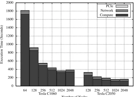
The graph in Figure 7 shows a breakdown of execution times for a Class E problem on different numbers of GPUs in terms of compute, network communication and PCIe transfer times. It is clear that the PCIe bus is not responsible for the poor scaling of LU. Furthermore, the network communication overhead is greater than that associated with the PCIe bus.

We identify two potential causes of the GPU implementa-tion’s limited scalability:

0 200 400 600 800 1000 1200 1400 1600 1800 2000

64 128 256 512 1024 2048 128 256 512 1024 2048

Ex

ecution

T

ime

(Seconds)

Number of Nodes

Compute Network PCIe

Tesla C2050 Tesla C1060

Fig. 7. Breakdown of execution times from the GPU model.

First, the 2D domain decomposition and strong scaling result in a decreasing amount of parallelism per GPU as the number of GPUs increase. The impact of this is greater for larger problem classes, as the height of each GPU’s tile-stack increases with problem size.

Second, the existingk-blocking policy trades GPU compute efficiency for pipeline fill time. A largekblockvalue is neces-sary to utilise the GPU’s parallel resources effectively (since it presents more parallelism), but this does not necessarily mean a decrease in execution time for the entire sweep. A larger

kblockis likely to take longer to process (which will increase the pipeline fill time) but also increases MPI message size (and larger messages may make more efficient use of network and PCIe bandwidth).

Thus, the scalability of this class of algorithm is impacted by device compute-performance; the SIMD width of the compute device; available memory per node; and network/PCIe latency and bandwidth. As CPU architectures become more SIMD-like (e.g through increased vector length) there is increasing need for these issues to be addressed.

A. Domain Decomposition

Under the 2D domain decomposition used in the original CPU implementation, ifNzincreases thenNx/PxandNy/Py must decrease in accordance with the memory limit of a node. This is significant because the size of a 3D grid’s largest hyperplane is bounded by the product of its two smallest dimensions – asNx/Px andNy/Py decrease, so too does the amount of available parallelism. A 3D domain decomposition would enable us to deal with an increase in Nz by adding more processors, thus preventing a decrease in parallelism.

Fig. 8. The newk_{-blocking policy.}

that the solution of a block of size Nx⇥Ny⇥Nz requires

Nx+Ny+Nz−2 wavefront steps.

As a corollary, a processor array of size Px⇥Py⇥Pz will have a compute time of:

(Px+Py+ ⇠

dNz/Pze

kblock

⇡

⇥Pz−2)W

whereW is the time a processor takes to compute a block of size Nx/Px⇥Ny/Py⇥kblock.

Thus an8⇥8⇥1processor array, with akblockof120, has a compute time of 22W, whereas a4⇥4⇥4 processor array, with akblockof240, has a compute time of10W. In order for the performance of the 3D decomposition to match that of the 2D decomposition, even when assuming zero communication cost, the value of W for a 240⇥240⇥240 block cannot be more than 2.2x greater than that for a120⇥120⇥120block. Our benchmarking reports that it is approximately 6x greater, demonstrating that a 3D decomposition does not result in a performance gain.

B. K-Blocking Policy

The k-blocking policy described earlier is very inefficient for values of kblock less than Nz. During the processing of each set of kblock tiles, the number of grid-points processed increases from 1towards some maximumH, before decreas-ing again to 1.

Ideally, we want to develop a method of k-blocking that allows us to process hyperplanes of sizeH in each wavefront step whilst having a minimal effect on the pipeline fill time and communication efficiency. Setting kblock=Nz produces the desired compute behaviour, but causes a considerable increase in pipeline fill time. Computing the values of all grid-points on the current hyperplane (even if they lie in the nextkblock) also increases parallel efficiency, but is complicated by the fact that the computation for some grid-points will depend on values yet to be received from processors upstream.

The reader is reminded that a single wavefront step moves from hyperplanef to(f+1); a single wavefront step increases the depth of the deepest grid-point the hyperplane intersects by one. Thus, a processor can execute s wavefront steps if

Nodes kblock Old Policy New Policy

4 1 759.99 80.81

81 67.25 77.13

8 1 554.34 74.94

41 52.92 61.34

16 ₄₁1 381.06_44.46 77.50_55.60

TABLE V

COMPARISON OF EXECUTION TIMES(IN SECONDS)FOR THE OLD AND NEWk-BLOCKING POLICIES.

and only if the data dependencies for all grid-points on the followings levels are satisfied; a processor receiving s rows or columns from those upstream can execute onlyswavefront steps.

This forms the basis for a newk-blocking policy, as depicted in Figure 8, which sees each processor running only kblock

wavefront steps upon receipt of a message. The end result of this policy is that the compute efficiency on each processor is maximised, at the expense of an increased pipeline fill time.

We present in Table V a comparison between the original

k-blocking policy and an early implementation of the new policy for a Class C problem executed on 4, 8 and 16 Tesla C1060 GPUs. In each case, the code was run with a kblock

of 1 (the best expected value for pipeline fill time) and

min(Nx/Px, Ny/Py)(the value used under the old policy). The results in this table demonstrate that the performance of the new policy is significantly better than that of the original policy for low values of kblock, yet slightly worse for high values. This is a direct result of the increased pipeline time.

In spite of this, our initial results show promise. That the performance of runs with low kblock values has been improved to such a degree demonstrates that the new policy will allow the value of kblock to be chosen based solely on PCIe and network latencies. We will investigate improvements to our new implementation and its effect upon the performance of large-scale runs in future work.

X. CONCLUSIONS

The porting and optimisation of parallel codes for accelerator-based architectures is a topic of intense current interest within the high performance computing community. This is in part due to the high levels of theoretical performance on offer from accelerator devices, as well as competitive levels of spatial and power efficiency.

assessment of LU’s performance on novel architectures to be published to date and provides insight into the performance of the code on alternative petascale-capable computing hardware. These results demonstrate that while distributed GPU clus-ters can deliver substantial levels of theoretical peak perfor-mance, achieving sustained application performance at scale is still a challenge. Like-for-like comparisons to existing technologies such as IBM’s BlueGene platform help also to show that the power-efficiency of GPU-solutions – a much cited reason for their adoption – is in fact comparable for this class of application.

These findings therefore raise interesting questions about the future direction of HPC architectures. On the one hand, we might expect to see smaller clusters of accelerator-based nodes which will favour kernels of highly vectorisable code; on the other, we might expect highly parallel solutions typified by the BlueGene/P, where “many-core” will mean massively parallel quantities of independently operating cores. Therefore, the choice that application programmers will be faced with is one of focusing on low-level code design (to exploit instruction-level and thread-instruction-level parallelism) or higher-instruction-level, distributed scalability.

This paper suggests that, for wavefront codes at least, both routes currently offer comparable levels of performance in spite of large differences in theoretical peak. The techniques employed in this work demonstrate a low-cost and accurate method of assessing application performance on contempo-rary and future high-performance computing systems – and emphasise the importance of consideringscale in application and machine design, in contrast to benchmarking on single nodes or small clusters.

ACKNOWLEDGEMENTS

This work is supported in part by The Royal Society through their Industry Fellowship Scheme (IF090020/AM). We are grateful to Scott Futral, Jan Nunes and the Livermore Computing Team for access to, and help in using, the Dawn-Dev BlueGene/P and Hera machines located at the Lawrence Livermore National Laboratory. Access to the LLNL Open Computing Facility is made possible through collaboration with the UK Atomic Weapons Establishment under grants CDK0660 (The Production of Predictive Models for Future Computing Requirements) and CDK0724 (AWE Technical Outreach Programme). The performance modelling research is also supported jointly by AWE and the TSB Knowledge Transfer Partnership grant number KTP006740. The authors would also like to thank the High Performance Computing team at the Daresbury Laboratory (UK) for access to the Daresbury multi-card GPU-cluster.

REFERENCES

[1] RNR-94-007 (1994) The NAS Parallel Benchmarks. NASA Ames Research Center. Moffet Field, CA.

[2] Mudalige, G. R., Vernon, M. K., and Jarvis, S. A. (2008) A Plug-and-Play Model for Evaluating Wavefront Computations on Parallel Architectures. Proceedings of the IEEE International Parallel and Distributed Processing Symposium, Miami, FL, 14-18 April. IEEE Computer Society, Los Alamitos, CA.

[3] Hammond, S. D., Mudalige, G. R., Smith, J. A., Jarvis, S. A., Herdman, J. A., and Vadgama, A. (2009) WARPP: A Toolkit for Simulating High-Performance Parallel Scientific Codes.Proceedings of the International Conference on Simulation Tools and Techniques, Rome, Italy, 2-6 March, pp. 19:1–19:10. Institute for Computer Sciences, Social-Informatics and Telecommunications Engineering, Brussels, Belgium.

[4] Hoisie, A., Lubeck, O., Wasserman, H., Petrini, F., and Alme, H. (2000) A General Predictive Performance Model for Wavefront Algorithms on Clusters of SMPs. Proceedings of the International Conference on Parallel Processing, Toronto, Canada, 21-24 August, pp. 219–228. IEEE Computer Society, Los Alamitos, CA.

[5] TR-08-24 (2008)Accelerating Data-Serial Applications on GPGPUs: A Systems Approach. Computer Science, Virginia Tech. Blacksburg, VA. [6] Munekawa, Y., Ino, F., and Hagihara, K. (2008) Design and Implementa-tion of the Smith-Waterman Algorithm on the CUDA-Compatible GPU. Proceedings of the IEEE International Conference on Bioinformatics and Bioengineering, Athens, Greece, 8-10 October, pp. 1–6. IEEE Computer Society, Los Alamitos, CA.

[7] Manavski, S. and Valle, G. (2008) CUDA Compatible GPU Cards as Efficient Hardware Accelerators for Smith-Waterman Sequence Align-ment. BMC Bioinformatics,9, S10.

[8] Petrini, F., Fossum, G., Fernandez, J., Varbanescu, A. L., Kistler, N., and Perrone, M. (2007) Multicore Surprises: Lessons Learned from Optimizing Sweep3D on the Cell Broadband Engine. Proceedings of the IEEE International Parallel and Distributed Processing Symposium, Long Beach, CA, 26-30 March. IEEE Computer Society, Los Alamitos, CA.

[9] Gong, C., Liu, J., Gong, Z., Qin, J., and Xie, J. (2010) Optimizing Sweep3D for Graphic Processor Unit.Proceedings of the International Conference on Algorithms and Architectures for Parallel Processing, Busan, Korea, 21-23 May, pp. 416–426. Springer-Verlag, Berlin. [10] (1995) ‘The ASCI Sweep3D Benchmark’. Los Alamos National

Lab-oratory. http://www.c3.lanl.gov/pal/software/sweep3d/sweep3d readme. html (12 May 2011).

[11] Boyer, M., Tarjan, D., Acton, S. T., and Skadron, K. (2009) Accel-erating Leukocyte Tracking using CUDA: A Case Study in Leveraging Manycore Coprocessors.Proceedings of the IEEE International Parallel and Distributed Processing Symposium, Rome, Italy, 23-29 May. IEEE Computer Society, Los Alamitos, CA.

[12] Govindaraju, N. K., Lloyd, B., Dotsenko, Y., Smith, B., and Manferdelli, J. (2008) High Performance Discrete Fourier Transforms on Graphics Processors.Proceedings of the ACM/IEEE Conference on Supercomput-ing, Austin, TX, 15-21 November, pp. 2:1–2:12. IEEE Press Piscataway, NJ.

[13] Shimokawabe, T., Aoki, T., Muroi, C., Ishida, J., Kawano, K., Endo, T., Nukada, A., Maruyama, N., and Matsuoka, S. (2010) An 80-Fold Speedup, 15.0 TFlops Full GPU Acceleration of Non-Hydrostatic Weather Model ASUCA Production Code. Proceedings of the ACM/IEEE International Conference for High Performance Computing, Networking, Storage and Analysis, New Orleans, LA, 13-19 November. IEEE Computer Society Washington, DC.

[14] Jacobsen, D. A., Thibault, J. C., and Senocak, I. (2010) An MPI-CUDA Implementation for Massively Parallel Incompressible Flow Computa-tions on Multi-GPU Clusters.Proceedings of the 48th AIAA Aerospace Sciences Meeting, Orlando, FL, 4-7 January. American Institute of Aeronautics and Astronautics, Reston, VA.

[15] Lee, V. W. et al. (2010) Debunking the 100X GPU vs. CPU Myth: An Evaluation of Throughput Computing on CPU and GPU. Proceedings of the ACM/IEEE International Symposium on Computer Architecture, Saint-Malo, France, 21-23 June, pp. 451–460. ACM New York, NY. [16] Vuduc, R., Chandramowlishwaran, A., Choi, J., Guney, M. E., and

Shringarpure, A. (2010) On the Limits of GPU Acceleration. Proceed-ings of the USENIX Workshop on Hot Topics in Parallelism, Berkeley, CA, 14-15 June. USENIX Association, Berkeley, CA.

[17] RC24982 (2010)Believe it or Not! Multi-core CPUs Can Match GPU

Performance for FLOP-intensive Application! IBM Research Division,

Thomas J. Watson Research Center. Yorktown Heights, NY.

[18] RC25033 (2010)Can CPUs Match GPUs on Performance with Produc-tivity?: Experiences with Optimizing a FLOP-intensive Application on CPUs and GPU. IBM Research Division, Thomas J. Watson Research Center. Yorktown Heights, NY.

of the NAS-LU Benchmark. SIGMETRICS Performance Evaluation

Review,38, 23–29.

[20] Lazou, C. (2010) ‘Should I Buy GPGPUs or Blue Gene?’. HPC Wire. http://www.hpcwire.com/hpcwire/2010-11-04/should i buy gpgpus or blue gene.html (04 November 2010).

[21] NAS-96-18 (1996)NAS Parallel Benchmark (Version 1.0) Results 11-96. NASA Ames Research Center. Moffet Field, CA.

[22] Ryoo, S., Rodrigues, C. I., Baghsorkhi, S. S., Stone, S. S., Kirk, D. B., and mei W. Hwu, W. (2008) Optimization Principles and Application Performance Evaluation of a Multithreaded GPU Using CUDA. Pro-ceedings of the ACM SIGPLAN Symposium on Principles and Practice of Parallel Programming, Salt Lake City, UT, 20-23 February, pp. 73– 82. ACM New York, NY.

[23] Lamport, L. (1974) The Parallel Execution of DO Loops.

Communica-tions of the ACM,17, 83–93.

[24] Gharaibeh, A. and Ripeanu, M. (2010) Size Matters: Space/Time Trade-offs to Improve GPGPU Applications Performance.Proceedings of the ACM/IEEE International Conference for High Performance Computing, Networking, Storage and Analysis, New Orleans, LA, 13-19 November. IEEE Computer Society Washington, DC.

[25] Reussner, R., Sanders, P., Prechelt, L., and M¨uller, M. (1998) SKaMPI: A Detailed, Accurate MPI Benchmark. Recent Advances in Parallel

Virtual Machine and Message Passing Interface,1497, 52–59.

[26] (2010) ‘Livermore Computing Systems Summary’. Lawrence Livermore National Laboratory. https://computing.llnl.gov/resources/systems summary.pdf (12 May 2011).

[27] Kerbyson, D. J., Hoisie, A., and Wasserman, H. (2005) A Performance Comparison Between the Earth Simulator and Other Terascale Systems on a Characteristic ASCI Workload. Concurrency and Computation: