Rochester Institute of Technology
RIT Scholar Works
Theses Thesis/Dissertation Collections
11-1-2008
Gamut extension algorithm development and
evaluation for the mapping of standard image
content to wide-gamut displays
Stacey E. Casella
Follow this and additional works at:http://scholarworks.rit.edu/theses
Recommended Citation
Gamut Extension Algorithm Development
and Evaluation for the Mapping of Standard
Image Content to Wide-Gamut Displays.
Stacey E. Casella
MUNSELL COLOR SCIENCE LABORATORY
CHESTER F. CARLSON CENTER FOR IMAGING SCIENCE
COLLEGE OF SCIENCE
ROCHESTER INSTITUTE OF TECHNOLOGY
ROCHESTER, NEW YORK
Accepted by:
Mark D. Fairchild, Advisor, M.S. Program Coordinator
Gamut Extension Algorithm Development and Evaluation for the
Mapping of Standard Image Content to Wide-Gamut Displays
Stacey E. Casella
ABSTRACT
ACKNOWLEDGEMENT
To my advisor, Dr. Mark Fairchild- Thank you for all of your support and guidance throughout my Master’s degree at RIT. I sincerely appreciate the opportunity you provided me to work on this thesis project. I have truly enjoyed the entire process, through which I have learned more than I ever expected.
I would like to express my sincere gratitude to Dr. Roy Berns for additionally providing me with the unforgettable opportunity to join the Color Science community. Also, thank you to the rest of the Munsell Color Science Laboratory faculty, present during my degree: Dr. Ethan Montag, Dr. David Wyble, Lawrence Taplin, Dr. James Ferwerda and Dr. Mitchell Rosen. I am reminded everyday in my professional career how much knowledge I obtained from all of you, and am incredibly grateful to have had that opportunity.
I also owe a special thanks to Dr. Rodney Heckaman. Rod—you kept me inspired throughout this program, bringing a smile to my face everyday. I owe much of my degree to your encouragement and support throughout my research, and am so fortunate to have your invaluable friendship to take with me. Also, to the two classmates I owe my survival of first year to- Shen and Nanette. We were an excellent team and I cannot express enough gratitude to both of you for all of your support. In addition, thank you to my best observer/recruiter –Erin. You helped me in so many ways this past year, taking my experiment and recruiting others, as well as being an excellent friend. Thank you to the rest of the Color Science family during my time at MCSL: Val, Colleen, Ben, Jonathan, Justin, Sunghyun, Abhijit, Philipp, Ying, Yang, Cathy, Tim, Mahdi, Mahnaz, Iris, Stefan, Susan, YK, to name a few! You all have provided me with such fond memories to remember my years at RIT by.
This research was made possible by Sony Corporation, in which I owe particular thanks to Masato Sakurai, Takehiro Nakatsue and Yoshihide Shimpuku for their guidance, contributions and cooperation throughout this collaborative research.
Table of Contents
1. Introduction... 1
2. Motivation: Wide Gamut Displays ... 2
3. Background ... 3
3.1 Gamut Mapping ... 3
3.1.1. Color Appearance Spaces ... 4
3.1.1.1. CIELUV ... 5
3.1.1.2. CIELAB ... 5
3.1.1.3. CIECAM97s ... 6
3.1.1.4. CIECAM02... 6
3.1.1.5. Rendering for accuracy ... 8
3.1.2. Compression Versus Expansion... 8
3.1.2.1. Compression Algorithms... 9
3.1.2.2. Expansion Algorithms... 14
3.1.2.2.1 Naturalness: An Influential Attribute... 15
3.1.2.2.2. Gamut Expansion Mapping in Various Color Spaces... 16
3.1.2.2.2.1. Establishing Colorfulness Boundaries ...17
3.1.2.2.2.2. Determining Influential Attributes ...18
3.1.2.2.3. Control Consideration ... 19
3.1.2.2.4. Gamut Expansion Linear Methods... 20
3.1.2.2.5. Gamut Expansion Non-linear Methods... 21
3.1.2.2.6. Gamut Expansion via a Mapping Direction ... 24
3.2 Extended Gamut Displays... 25
3.2.1. LCD with LED Backlight ... 26
3.2.1.1 Sony Prototype, 40 inch, LED backlit, 1080p, LCD ... 28
3.2.2 DLP with LED primaries ... 29
3.2.2.1 Samsung HLT5087s, 50 inch, slim LED Engine, 1080p, DLP... 31
3.3 Display Color Spaces... 34
3.3.1. sRGB Color Space... 35
3.3.2. YCC Color Space ... 37
3.3.2.1. Sensitivity of the Human Visual System to Luminance and Chrominance ... 37
3.3.2.2. Chromaticity Gamut Area of YCC Color Space ... 38
3.3.2.3. The premise of YCC ... 40
3.3.2.4. ITU Existing Standards ... 43
3.3.3. Expanded Gamut Color Space (xvYCC) ... 44
3.3.3.1. Gamut Area of xvYCC... 44
4.1.1. One-Dimensional LUT ... 48
4.1.1.1 Sony Display ... 50
4.1.1.2 Samsung Display ... 50
4.1.2. Three-dimensional LUT... 60
4.2 Experimental Conditions: Dim Versus Dark Surround ... 64
4.2.1. The Effects of Dark Surround ... 66
4.2.1.1. Stimuli... 66
4.2.1.2. Experimental Methods ... 66
4.2.1.3. Results and Discussion... 69
4.3 Methodology ... 79
4.3.1. Viewing Conditions and Observations ... 79
4.3.2. Stimuli... 81
4.4 Algorithms ... 85
4.4.1. Background ... 87
4.4.2. Linear Algorithms (LGEAs) ... 88
4.4.3. Sigmoidal (Nonlinear) Algorithms (SGEAs)... 102
4.4.3.1. Reference Point Extension ... 111
5. Data Analysis... 120
6. Conclusions ... 135
List of Figures
Figure 3.1. CIELAB coordinates of OSA color scales sampling. ... 7
Figure 3.2. CIECAM02 coordinates of OSA color scales sampling ...7
Figure 3.3 Core gamut boundary on L-C plane ... 12
Figure 3.4. Red, Green and Blue LEDs [P.Namek, Wikipedia, 2008] ... 26
Figure 3.5 A subpixel in a LCD [M. Raaijmakers, Wikipedia, 2008]... 27
Figure 3.6. Simulated depiction of LCD pixels operating together to display an image [V. Ezekowitz, Wikipedia, 2008]... 28
Figure 3.7 Red, Green and Blue primaries for the display gamut (Sony) and the input (sRGB) gamut. ... 29
Figure 3.8. DMD representation... 29
Figure 3.9. Microscopic mirrors within DLP device. ... 30
Figure 3.10. Process of projecting an image on a DLP HDTV with LED illumination [TI; 2008]... 30
Figure 3.11 Chromaticity gamut areas of the two destination gamuts: Samsung and Sony displays, in comparison to sRGB. ... 32
Figure 3.12. The luminance values, of the red channel, from tristimulus measurements for multiple contrast/brightness combinations... 33
Figure 3.13. Chromaticity diagram with labeled white points from the measured color tone settings, as compared with D65... 34
Figure 3.14. Gamut areas of sRGB, YCC and their newly developed, wide-gamut color space, xvYCC [Matsumoto et al., 2006]. ... 39
Figure 4.1. Chromaticity diagram with primaries from both SN and MW modes... 51
Figure 4.2. Measured tristimulus values converted to chromaticity coordinates, corresponding to the red, green and blue ramp data. ... 52
Figure 4.3. Three one-dimensional look-up tables derived from the measured tristimulus values of the RGB ramps and neutral data. ... 53
Figure 4.4. 100 randomly generated colors on a chromaticity diagram... 54
Figure 4.5. CIEDE2000 color difference histogram for the randomly generated set of 100 samples. ... 56
Figure 4.6. Comparison of estimated CIELAB values with the measured CIELAB values, where the arrows run from the measured to estimated values. ... 57
Figure 4.7. CIELAB vector plot for a second randomly generated sample set, where the arrows run from the measured CIELAB values to the estimated values... 58
Figure 4.8. Luminance values of the RGB ramps added together compared with the equal digital count ramp (R=G=B)... 59
Figure 4.12. CIELAB vector plot representing each of the 100 samples, with color difference arrows representing the magnitude of CIEDE2000 and direction towards
the estimated values... 62
Figure 4.13. Color difference histogram of white, black, red, green, blue, yellow, cyan, and magenta color patches... 63
Figure 4.14. CIEDE2000 color differences for the gray, red, green blue generated ramps in addition to the white, black, red, green, blue, yellow, cyan and magenta colors.. 63
Figure 4.15. a. Original sRGB flower image... 64
Figure 4.15. b. Reproduction of flower image under 3DLUT characterization. ... 64
Figure 4.16. a-c. (a) Coast Image, (b) Musicians Scene, (c) Flowers image. ... 66
Figure 4.17. Simulated primaries in xy chromaticities for a color gamut volume factor of k = 1.0(a), 0.8(b), 0.6(c), 0.4(d) and within each plot, a lightness contrast factor of kLC of 1.00, 0.875, 0.75, 0.625 times the full, extended gamut of the display ...68
Figure 4.18: Perceived colorfulness as a function of the percentage of NTSC color gamut area in xy chromaticities for each log contrast ratio, for the flower scene averaged over eight observers for Experiment IIIb and six observers for Experiment III... 69
Figure 4.19: Contours of equal colorfulness, determined by multiple linear regression, as a function of percentage of NTSC color gamut area in xy chromaticities and log contrast ratio, for Experiment III (solid) and Experiment IIIb(dotted), averaged over observers, for the flower scene. ... 70
Figure 4.20: Lightness contrast interval scores as a function of the percentage of NTSC color gamut area in xy chromaticities for each log contrast ratio evaluated, for the musician scene from both Experiment III and the dark room experiment. ... 71
Figure 4.21: Lightness contrast in terms of category scores as a function of color gamut volume for each of the four log contrast ratios, for the coast scene... 73
Figure 4.22: Fitted contours of equal lightness contrast as a function of percentage of NTSC color gamut area in xy chromaticites and log contrast ratio, for the coast scene. ... 74
Figure 4.23: Both Experiment III and Experiment IIIb represented in an interval score plot for preference as a function of percentage of NTSC color gamut area in xy chromaticities and log contrast ratio, for the musician scene. ... 75
Figure 4.24. Preference interval scores, as a function of percentage NTSC color gamut area in xy chromaticities and log contrast ratios for the flower scene in both Experiments III and IIIb. ... 76
Figure 4.25: Fitted contours of equal preference interval scores as a function of percentage NTSC color gamut area in xy chromaticities and log contrast ratio, for the flower scene from Experiments III and IIIb... 77
Figure 4.26. Experimental set-up for both displays... 80
Figure 4.27. Lady image... 81
Figure 4.28. Musician scene. ... 81
Figure 4.29. Water image. ... 82
Figure 4.30. Coast scene... 82
Figure 4.31. Florent Tetons image... 82
Figure 4.32. Flower image... 83
Figure 4.35 Fog image. ... 84
Figure 4.36 PW837_rgb. ... 84
Figure 4.37 Flowchart converting digital counts under sRGB color space, to RGB digital counts corresponding to the display, representing the first baseline version. ... 86
Figure 4.38. Flowchart representing the second baseline image, where the input digital counts were directly sent to the output device and displayed... 87
Figure 4.39. At multiple hue angles, the maximum chromatic values are computed for given lightness values for both the input (sRGB) gamut and destination (SONY and Samsung) gamuts. ... 92
Figure 4.40. The transformations of all three LGEAs for the Sony display at various hue angles. The lines extend from sRGB chroma values to expanded chroma. Note: the color of the data corresponds to the appropriate hue angle. ... 97
Figure 4.41. The transformations of all three LGEAs for the Samsung display at various hue angles. The lines extend from sRGB chroma values to expanded chroma. Note: the color of the data corresponds to the appropriate hue angle... 100
Figure 4.42. The three sigmoidal curves applied to this study are based on Eqn. 4.11. The red curve represents SGEA1, the blue curve represenets SGEA2 and the cyan curve represents the third SGEA... 103
Figure 4.43. The chroma transformations of the three sigmoidal transfer functions (SGEA1-left, SGEA2-center, SGEA3-right. The lines extend from the original sRGB chroma values to the Sony expanded. Note: the color of the data corresponds to the appropriate hue angle... 107
Figure 4.44. The chroma transformations of the three sigmoidal transfer functions (SGEA1-left, SGEA2-center, SGEA3-right. The lines extend from the original sRGB chroma values to the Samsung expanded values. Note: the color of the data corresponds to the appropriate hue angle. ... 110
Figure 4.45. Constant Lightness with sigmoidal gamut expansion ... 111
Figure 4.46. Sigmoidal gamut expansion away from L*=50, or mid-gray... 111
Figure 4.47. Sigmoidal gamut expansion away from L*=0, or black... 111
Figure 4.48. The expansion of one specific pixel where the expansion is extending from L*=50 ... 112
Figure 4.49. The transformations of sRGB values, corresponding to the Sony display output values, for hue angles between 270 and 275. The most left plot is constant lightness, the center extends from L*=50 and the right plot extends from L*=0... 114
Figure 4.50. The transformations as a result of SGEA1LC andSGEA1L50, corresponding to the Sony display, for a range of hue angle (the color of the data corresponds to the applicable hue angle)... 116
Figure 4.51. The transformations as a result of SGEA1LC and SGEA1L50, corresponding to the Samsung display, for a range of hue angles (the color of the data corresponds to the applicable hue angle). ... 118
Figure 5.3. The Lady bar plot in interval scores, which directly correlate to overall observer preference. These data are representative of the average observer’s
response. ... 125 Figure 5.4. The musician image results represented as interval scores for the average
observer. ... 126 Figure 5.5. The flower scene preference results for each of the eleven algorithms, and
both Sony and Samsung displays, are displayed for the average observer. ... 128 Figure 5.6. Fluorent Tetons results, averaged across observers, for each algorithm,
displayed for both devices. ... 129 Figure 5.7. The preference results for the barn image for each algorithm and both display evaluations, average across observers. ... 130 Figure 5.8. The coast scene is represented in terms of interval scores of preference.... 131 Figure 5.9 Sample transformations under SGEA1L50 for hue angles between 170-175.
... 132 Figure 5.10. Preference interval scores for the fog image, for each of eleven algorithms
List of Tables
Table 3.1. Controllable display options and the combinations chosen for analysis. ... 33
Table 4.1. Curve characteristics of the sigmoidal functions represented in Figure 4.42. ... 103
Table 5.1 Interval Score calculations for Sony evaluation... 123
Table 5.2 Interval Score calculations for Samsung evaluation ... 123
Table 5.3 Rank order for Sony evaluation ... 124
1. Introduction
2. Motivation: Wide Gamut Displays
A collaborative, necessary effort between Sony’s Standard Systems Development Department, Sony Corporation, and the Munsell Color Science Laboratory (MCSL) at the Rochester Institute of Technology (RIT) focused on enhancement of digital image content under existing standards by exercising wide color gamuts. This research will provide guidance on the enhancement of image content, so that both the production and consumption sides of the display industry will benefit. Specifically, the aim of this research is to devise a gamut expansion strategy that is most visually pleasing to the average observer.
3. Background
The display technology facilitates the rendering capabilities under the given GEAs. Therefore, it is necessary to fully understand the limitations due to the display itself in order to provide greater opportunity to incorporate a successful mapping strategy.
3.1 Gamut Mapping
The phrase, “a picture is worth a thousand words,” stems back to an article written by Fred Barnard in 1921, although increases in value still today. Imagery enables stories to be told, concepts to be made, and even, surgeries to be conducted. Technology has certainly aided this proverb throughout the years, and continues to have a large influence over images. With the introduction of digital photography, for example, cross-media processing can easily take place. However, working with different media introduces new challenges.
With each type of device, and each company responsible for designing and producing the devices, different specifications are set. Therefore, when converting data formulated for one device to a second device, it is necessary to bring the data in sync with the latter device’s specifications so that the image will look reasonable. This happens to be a complicated process in the color field.
representation on a chromaticity diagram, as this does not account for varying luminance. Therefore a “gamut” depicted on a chromaticity diagram will be noted as a chromaticity gamut.
Typically in the situation where an image is obtained on an input device, and converted to an output device, there are three unique gamuts involved: the input, output and image gamut [Stone et al.; 1988]. Therefore, when information is transferred between devices, the image gamut is correspondingly adjusted based on the rendering intent: generally the objective is to obtain either the most accurate, or most preferable reproduction. Once the image has been rendered, this reproduction will correspond with the output device, as desired.
Despite the details behind the mapping, color appearance attributes guide the transformation between spaces. Considering a display, without considering the appearance attributes of that display is meaningless. Therefore, an optimal color space to perform color transformations would be a color appearance space, as this space would be “perceptually meaningful” [Fairchild; 2005]. Using a color appearance space allows lightness, chroma and hue to be manipulated independently, so the input gamut can be mapped in the best possible manner. There are several color appearance spaces, however, to choose from.
3.1.1. Color Appearance Spaces
Fairchild; 1998). However, prior to these references and other research that incorporated results from both CIELAB and CIELUV, there were several gamut mapping algorithms designed using CIELUV color space.
3.1.1.1. CIELUV
CIELUV as a color appearance space intuitively made sense; CIELUV space was theoretically perceptually uniform, and therefore, was expected to make a good color appearance space. Wolski et al., 1994, chose CIELUV over CIE’s XYZ, xyY, and CIELAB based on the perceptual uniformity characteristics of the spaces [Wolski et al.; 1994]. In addition, Gentile et al. noted CIELUV provided a better space to conduct gamut mapping methods under (“color gamut mismatch compensation”) compared to RGB [Gentile et al.; 1990]. Therefore, when choosing from limited color spaces to begin with, CIELUV seemed to be the best available space resembling a color appearance type space. There were a variety of best-performing algorithms, however, Wolski et al. concluded that different areas of the color space resulted in different preferred mapping directions [Wolski et al.; 1994]. Due to the lack of consistency amongst results, research began to focus on other color appearance spaces in search of a more reliable results.
3.1.1.2. CIELAB
despite the ability of CIELAB to be used as a color appearance space, perceived hue is not linearly related to lines of constant metric hue angle [Braun, Fairchild and Ebner; 1998]. As a result, although CIELAB performs well in areas excluding the blue region, this region proved reason enough to explore gamut mapping in other color appearance spaces.
3.1.1.3. CIECAM97s
Prior to 2002, CIECAM97s was the latest and most robust color appearance space that existed; it was recommended by the CIE committee in 1997 as a means for describing color appearance while defining cross-media conditions. Although CIECAM97s required some revisions and improvements (predominantly in regard to simplification), this color space far surpassed CIELAB and CIELUV in terms of describing the working conditions of conversions occurring cross-media.
Morovic and Luo performed an evaluation of specific gamut mapping algorithms in CIECAM97s, given the uniformity of the hue predictor was improved from that under CIELAB. They reported that the blue region performed significantly better using CIECAM97s because of the hue nonlinearities prevalent in CIELAB for this region. However, CIECAM97s resulted in hue shifts in the red/yellow range, an effect absent from the results under CIELAB. Overall, the results from CIECAM97s were comparable to the previously made CIELAB manipulations, with varying advantages and disadvantages.
3.1.1.4. CIECAM02
dependence in absolute luminance). In addition, CIECAM02 improves hue constancy significantly. In Moroney and Zeng’s article, “Field trials of CIECAM02 color appearance model” published on Hewlett Packard’s website, both CIELAB and CIECAM02 coordinates of OSA Color Scales are represented in Figures 3.1 and 3.2.
The improvement of hue linearity for CIECAM02, compared to CIELAB, is quite evident through Figures 3.1 and 3.2. In these figures, color scales in the applicable color space are represented, where lightness increases into the page. The color scales break down in Figure 3.1 under CIELAB in the blue region, whereas this is significantly improved under CIECAM02.
In all of the above research conditions, a common conclusion was drawn: the output reproductions resulting from gamut mapping were dependent on the appearance space used. In addition, another factor is the intent of the gamut mapping. As mentioned above, two clear distinctions were either obtaining an accurate reproduction, or a most pleasing rendering. Each rendering intent is a unique motive for the gamut mapping algorithms.
Figure 3.1. CIELAB coordinates
3.1.1.5. Rendering for accuracy
Obtaining an accurate color appearance to the original proved to be challenging. Morovic and Luo attempted to find a universal, robust gamut mapping algorithm that provides the most accurate color reproduction. More specifically, enhancement was not desired. Both CIECAM97s and CIELAB were incorporated into a psychophysical analysis, so that a comparison between the two methods could be made. The gamut mapping algorithms incorporated lightness and/or chroma compression, while preserving hue. There were five specific algorithms evaluated, each that performed specific operations relative to the output gamut size.
A few observations were made; CIECAM97s resulted in wider lightness contrast ratios than CIELAB did. Since the output gamut was smaller than the original gamut, a prevalent consequence of compression is loss of lightness contrast. However, to retain the original look, it is important to retain as much of the lightness contrast as possible. Therefore, based solely on this reasoning, one may predict the CIECAM97s manipulations would better resemble the original. However, the authors reported similar results between the two color spaces, as noted above. In addition, Morovic and Luo found it more critical to maintain chroma, even when that meant perceived lightness takes the hit. In addition, the most accurate renderings resulted from the algorithms that affected the perceptual attributes the least. And so, without many solid conclusions, gamut mapping remains the key focus.
rendering intent, as well as the individual device gamuts involved. The output gamut size relative to the input gamut takes a large toll on the design of the GMA. Historically, compression explained every GMA. However, with the new technology available today, compression in many cases is no longer applicable. Gamut expansion has become of interest with the introduction of the new technology as color becomes a large focus for displays. Imagery has in the past, and continues to strive to represent what the human visual system can perceive. Therefore, color management has become a high priority in display devices. Hence, with better display capabilities comes the ability to display a greater range of colors. Although compression may no longer be the focus of GMAs, these algorithms serve as an excellent baseline to derive gamut mapping methodologies.
3.1.2.1. Compression Algorithms
Many GMAs are designed for compression due to the limited output gamut size. It is clear that a reproduction resulting in reduced color and reduced lightness contrast is no longer a goal; however, with a limited output gamut volume, this may become the inherent result.
When mapping is conducted in color appearance spaces, and thus, perceptual attributes are manipulated, it proves valuable to perform psychophysical experiments on the rendered images to determine the strategies that resulted in the best reproductions. Gentile et al. studied color gamut mismatch compensation in 1990, where their focus was on creating brighter, more colorful colors in both display and printing applications: a focus that is still, eighteen years later, a high priority.
of the relationship between colors. Compression works harder to retain the general relationships, and therefore, may compress the attributes more than necessary in doing so [Gentile et al.; 1990]. Thus, they found clipping was preferred unanimously. In addition, the algorithms that preserved lightness, or lightness and hue attributes in combination, were consistently preferred as well. Overall, the best performing algorithm clipped chroma, while maintaining lightness and hue.
Similarly, Wolski et al., 1994, investigated compression techniques and noted global compression resulted in a loss of lightness contrast. A soft compression technique was implemented to bypass this negative consequence. The conclusions, supported by the results from previous research, focused on the significant image and color space dependencies. The technique introduced in this article focused on incorporating these dependencies into an automatic algorithm for gamut mapping. This algorithm considered the color coordinates within the specified color space, and manipulated those coordinates correspondingly. The goal was to design a computer-generated, universal algorithm that could incorporate specific attributes of an image into the process. In the end, the authors were not convinced that the one universal algorithm sought out for is even attainable. It seemed the image dependencies may be too large to create the versatile algorithm intended.
artificial boundary conditions. Again, the most preferred method maintained hue and lightness, and clipped the out-of-gamut chroma coordinates.
When Montag and Fairchild, 1998, evaluated chroma clipping for three unique output gamuts, hue and lightness dependencies were prevalent. The best method varied depending on the lightness extremes (top or bottom of the gamut). At the higher lightness values, a soft-clipping or knee compression function applied to lightness values was preferred such that chroma was reduced to maintain constant saturation. In contrast, the darker regions were rendered well under clipping of the lightness values to maintain saturation. Overall, for lightness mapping, it was critical that saturation was maintained. This was not the case for chroma mapping, however. Straight clipping was preferred for this mapping, as other studies have shown as well.
In 2000, Braun and Fairchild developed algorithms for gamut mapping that again, incorporated soft-clipping or knee-functions. These functions make a slower transition to the output gamut, compared to clipping or straight compression. The reported results correlated well with previous studies: compression caused an undesired, dramatic change. The linear lightness compression resulted in lighter renderings that displayed lower contrast. In addition, the linear chromatic compression reduced chromatic contrast, and as a result, flesh tones appeared washed out. Using a soft-clipping or knee-function allowed the transformation to take place gradually, so that lightness and chromatic contrast was maintained from the original.
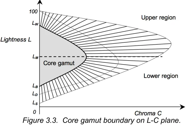
boundary (Figure 3.3) on the lightness/chroma plane such that, colors within the boundary were held constant. Mapping was only applied to those colors outside the core gamut boundary as an effort to maintain low chromatic colors. The core gamut boundary was defined so that the cusp was located at the lightness value that corresponded to the destination gamut cusp. Then, using a chroma-scaling constant, generally between 0.7 and 0.9, the core boundary was defined [MacDonald et al.; 2000].
[image:23.612.142.442.438.642.2]In addition to the defined core boundary, the algorithm incorporated a bilinear function. This function extended colors outside of the core along the designated mapping directions to the destination gamut, according to the range of lightness values the coordinate fell into. This method, in addition to three other GMAs comprised of varying techniques, was psychophysically evaluated. Although the topographical method was ranked high, MacDonald et al. noted important improvements necessary in order to increase the GMA’s performance.
GMA had both the core gamut and destination gamuts “coterminous” at a lightness value of 100. In addition, the mapping chords were comprised of a soft-clipping function to accommodate the colors outside the source gamut boundary. These alterations dramatically improved the results, as this topographical method was now most preferred by observers when compared with the same three algorithms.
Obvious trends in the above studies have become apparent through this review. Much of the research conducted on gamut mapping strategies often manipulates similar attributes, while maintaining others. Since a universal gamut mapping algorithm is an important goal, specific manipulations can be noted in which should be included in a final algorithm.
The most pronounced objective, common among many researchers, is the requirement for constant perceived hue. Unfortunately, perceived hue often does not directly correlate to constant metric hue. Some appearance spaces are better than others in this respect, and thus, this objective is limited to the capabilities of the color space chosen for manipulating the data. In addition, the range of lightness and colorfulness, or achromatic/chromatic contrast, should be preserved if possible. By maintaining both lightness and colorfulness contrast, the relationships between objects within the image can be retained, thus, preventing a decrease in preference. In addition, maintaining a constant saturation was found to influence observer preference. By preserving saturation, particularly in regions of low chroma, the appearance of a “washed out” image or desaturated features was avoided.
mapping algorithms is largely dependent on both the color space and image content, improvements are still currently of interest to encompass more images and conditions.
The research described above presents a range of alternatives to mapping image content to a smaller gamut (often to the gamut of a printer), and thus, incorporated both clipping and compression techniques. However, with the addition of wide-gamut display technology, the focus is aimed toward gamut mapping algorithms used to expand the input image content. This objective is newer, however, progress has already been made.
As previously mentioned, Fedorovskaya et al., 1996, evaluated perceptual quality, colorfulness and naturalness for reproductions created through chroma variations on multiple scenes. The results displayed a direct correlation between perceptual quality and naturalness, however, the more profound conclusion from this study entailed colorfulness. Colorfulness was found to be the most significant factor effecting image quality, out of the two evaluated.
3.1.2.2. Expansion Algorithms
manipulating color appearance attributes, and can now be incorporated into the research conducted on expanding the input gamut.
Now that gamuts are getting wider, the issue has changed from gamut compression to gamut expansion. However, applying the knowledge gained from the former objective can aid in the research towards establishing a robust gamut expansion algorithm.
3.1.2.2.1 Naturalness: An Influential Attribute
The complex nature of color is a result of the uniqueness of human visual perceptions. For imagery purposes, color variations have been studied for both quality and preference as an effort toward creating more visually satisfying images. Fedorovskaya, Ridder and Blommaert (1997) evaluated the effects of chroma variations, in CIELUV color space, within natural scenes on perceptual quality, colorfulness and naturalness. As previously mentioned, gamut mapping algorithms are driven by one of two motives: accuracy or pleasantness. In other words, if an algorithm is driven toward accuracy, the reproduction may not necessarily be the most preferred. Similarly, if an algorithm is based on preference, the result may not be accurate according to the spectral properties of the objects within the image. This is largely influenced by memory colors, and the fact that the average observer sees given memory colors as a specific color name, regardless of the illumination of the scene or spectral properties of the objects.
Fedorovskaya et al. claim an observer inherently compares the scene at hand with an “internal reference” or “memory representation”. Therefore, an image worthy of high image quality ratings must be perceived as natural. Ridder and Blommaert concur that the naturalness of an image, which largely affects image quality, also depends on the familiar memory colors. Most research conducted on gamut mapping algorithms has focused on mapping complex images, and therefore, generally the scenes are of natural context (one notable exception will be discussed later [Laird and Heynderickx; 2008]).
3.1.2.2.2. Gamut Expansion Mapping in Various Color Spaces
Color has two attributes: saturation and chroma. In a natural scene, all objects are similarly illuminated, and therefore, saturation remains constant since the objects in the scene are present under the same reference white. However, maintaining a constant hue and lightness over two uniquely colored regions results in color differences due to chroma variation (Eqn. 3.1.), in CIELUV space [Federoskaya et al. 1997].
!
"E*UV =
[
(
"L*)
2+(
"H*)
2+(
"C*)
2]
(3.1)influenced image quality and naturalness more so than chroma variations [Ridder and Blommaert; 1995]. Therefore, both hue and chroma are critical color attributes that influence color reproduction.
3.1.2.2.2.1. Establishing Colorfulness Boundaries
To this, technology has caught on, as it did not take long before the market was inundated with extended gamut displays. Given the importance of color in the processing chain, it only made sense to obtain the most colorful reproduction possible, using the display primaries as the limiting factor. However, the naturalness of an image became of utmost importance, after the images were not performing as expected. To evaluate this further, Laird and Heynderickx evaluated perceptually optimal boundaries and reported an intriguing conclusion about gamut expansion algorithms.
While Laird and Heynderickx discussed the advantages of the current technological advancements in wide-gamut televisions, they also noted that regions of “very intense, bright colors” can be “displeasing” to observers. Using scenes of limited content, predominantly monochromatic in color, and unrelated to memory colors, observers adjusted chroma for given hue and lightness values until the scene appeared unnatural. The purpose was to describe a perceptually optimal boundary within CIELAB space in which, a gamut extension algorithm should not exceed.
3.1.2.2.2.2. Determining Influential Attributes
In their evaluation, Kang et al. implemented a computer-controlled, interactive tool that enabled the observer to adjust color regions within a given area to represent a more preferred color reproduction. The observers were first trained to understand lightness, chroma and hue attributes, and then were allowed to manipulate certain color regions within the image content. This method enabled algorithm development designed specifically on the data supplied by the observers.
Based on the first round of experiments, the data supported the conclusions that the algorithm should not incorporate a hue shift. Since the observers did not alter the color region to a significantly different hue, this attribute was not varied within the algorithm. An encouraging result became clear through the second part of the experiment: after observers altered the images, a GEA was developed. In addition, four unique GEAs were developed by varying the degree of chromatic extension, where all were then compared through an overall preference experiment. The results indicated that the extensions applied by the observers in the first experiment were insufficient, in that more dramatic chromatic extensions were preferred when later evaluations were conducted. Therefore, observers actually preferred more colorful images than they originally created. Despite the conclusion Laird and Heynderikx reported, Kang et al. found support for wide gamut technology.
impact GEA preference, and thus, should be considered in the algorithm development stages.
An additional consideration to algorithm development should be dynamic range. With the introduction of wide gamut technology comes larger dynamic ranges. In addition to incorporating increased colorfulness into GMAs, Reinhard et al., 2007, remark on the importance of creating GMAs that correspond to high-dynamic range displays. The radical difference between real world illumination and the capabilities of current gamut mapping strategies emphasizes the journey researchers still have to bring these closer together. Reinhard et al. explain that maintaining equal or greater dynamic ranges within a given image content will better ensure success of the reproduction.
3.1.2.2.3. Control Consideration
When analyzing GEAs, it is important to validate the necessity of expanding the gamut from the current EBU standard. Therefore, Muijs et al. (2008) included a true-color representation of the test images in their psychophysical study evaluating observer preference for gamut extension algorithms. A true-color representation displays an EBU input image correspondingly on a wide-gamut display. By accounting for the difference between the input and display primaries, the image is displayed on a wide-gamut monitor within the input gamut. This version serves as a baseline image as it is not expanded beyond the EBU standard.
display gamut. This theoretically represents a more colorful image. However, this reproduction largely depends on the display technology, and has the potential to drastically alter the overall image appearance. By incorporating true-color representation and the linearly stretched version as the two mapping extremes, proper comparison and analysis of any developed gamut expansion strategies is enabled.
Similar to gamut compression algorithms, GEAs can entail multiple color appearance spaces to perform mapping in. However, the correlation between chroma and colorfulness guides the decision of what space to perform the mapping in. CIELAB is the most common color space GEAs are performed in because it is a perceptually meaningful color space in which, chroma can easily be both calculated and manipulated [Muijs et al.; 2008, Kotera et al.; 2002, Kotera et al.; 2001, Kang et al.; 2005, Kang et al.; 2003, etc.].
Kang et al., 2005, provide an overview to demonstrate the variety among mapping algorithms incorporating CIELAB space. These methods are based on CIELAB attributes, such that both lightness and chroma are mapped using multiple functions. They discuss both linear and non-linear mapping functions as methods conducted in past research. These functions enable a mapping to incorporate attribute dependencies so each CIELAB coordinate is mapped appropriately. This becomes particularly useful when considering memory colors (i.e. skin, blue sky and green grass [Kang et al.; 2005]), as these are fairly unique color regions that need to be carefully mapped in order to satisfy the observer.
coordinates by incorporating the ratio of the input to output lightness ranges. After calculating the range between the maximum and minimum lightness values for both the input and destination gamut, a ratio between the ranges was obtained. Using this ratio, the expanded, output chroma, C2 was calculated from a line that was formed between (L1,
C1) and (L2, C2) such that hue was maintained. Therefore, by constraining hue, and using
the ratio of dynamic ranges for each gamut, Hoshino successfully linearly expanded the input data to a larger gamut. This concept of mapping lightness/chroma coordinates showed great potential and thus, is commonly incorporated into gamut expansion evaluations.
3.1.2.2.5. Gamut Expansion Non-linear Methods
Muijis et al., 2008, developed three methods (one-linear, two-non-linear), all of which manipulated lightness and/or chroma values to extend along a given direction with a given driving function. One of the methods, denoted wide gamut color mapping, WGCM, was derived as a linear combination of both the true-color mapping and the linearly stretched mapping, where the output was dependent on the input saturation. The idea behind the dependency on saturation was to maintain neutral colors while drastically enhancing highly saturated colors. Through this method, colors of low saturation could retain a reasonable color, while the more chromatic colors were enhanced, so that the full display gamut was utilized.
varied both chroma and lightness in a lightness-dependent manner, while maintaining hue. Thus, the latter accounted for variations in lightness, particularly at the extremes. As a result, this method balanced contrast enhancement for the bright and dark, low saturated, near-neutral colors with the mid-lightness, highly saturated, chromatic colors [Muijs et al.; 2008].
Through their psychophysical analysis, the only method out of the three developed that was significantly preferred over the true-color mapping was the lightness/chroma mapping. At the lightness extremes, a device’s color gamut varies drastically in comparison to mid-lightness values, as typically mid-lightness values enable more chromatic colors to be reproduced. This mapping took this into account by varying the degree of extension based on the lightness values. This was done through a sigmoidal transfer function so that different chroma/lightness combinations resulted in different extensions. Therefore, this method enabled special consideration for memory colors.
resulted in a higher user satisfaction index (USI) than the standard mapping solution. This is because in this case, there was additional consideration taken for the expansion methods of specific color regions. The non-linearity of the method enabled a greater degree of specificity for individual color regions, which was highly received according to the observer data.
Simliar to Bang and Choh, Anderson et al., 2007, employed a nonlinear method to avoid the oversaturation of specific color regions (i.e. skin tones, pastels and neutrals) as a result of linearly mapping to an extended destination gamut. Using extended color pair samples provided by color experts, for a given image frame, local linear regression was performed and applied to the scene using multi-dimensional look-up-tables stored in an ICC profile. Based on past research that suggested any GMA developed is inherently image-dependent, Anderson et al. felt this was a reasonable mechanism to better automate the process. Video and image sets were incorporated into the experiment, each with four versions: original, expanded, linearly expanded and mapped via a locally linear LUT. Hue dependencies were evident through the results, however, the locally linear LUT clearly outperformed the other methods. Still, this regression technique was costly since the ground truth from the artistically expanded color pairs was necessary for each individual image set. Therefore, the regression technique has not been actively pursued as of yet.
Therefore, they performed a Gaussian histogram on the luminance channel, and followed with separating the chrominance components according to luminance and hue angle. The chroma of each value was then extended by the Gaussian histogram, while maintaining hue. This type of gamut algorithm is an automated approach to an image-dependent algorithm. Therefore, this is a method to use in place of the development of a cumbersome image-dependent algorithm, and as a result, it has more potential to be accepted as a standard GMA than it otherwise would have had.
3.1.2.2.6. Gamut Expansion via a Mapping Direction
Aside from the general basis behind the GEA (linear or sigmoidal), an additional consideration should be taken to address the direction of the mapping. MacDonald et al., 2001, commented on directional mapping for compression toward a specified cusp, given their mapping chords were required to be defined extending to and from specific directions. Kang et al., 2005, distinguish between mapping function and direction in their description of chroma mapping. Maintaining a constant lightness is common amid past research [Montag and Fairchild; 1996, Gentile et al.; 1990, Morovic and Luo; 2001, Wolski et al.; 1994]. In addition, however, mapping to/from a specified point can also prove very useful.
coordinates increased. However, with gamut expansion, in which, mapping would extend away from the anchor point, this was not an issue. This method, therefore, served as an excellent baseline, which was further expanded on to include a second variable point to be evaluated. Overall, the SGEAs were evaluated extending from L* equal to zero, L* equal to fifty, in addition to maintaining lightness values.
3.2 Extended Gamut Displays
Gamut mapping algorithms that extend the input color values become pertinent for extended gamut displays. The limitation of enhanced color reproductions is dependent on the gamut of an extended-gamut display. Current technology boasts expanded primaries, thanks to the advancement of light-emitting diodes (LEDs). Since 2006, LEDs have become increasingly prevalent in a number of technologies, gaining advocates for their increased color output and efficiency.
In regard to displays (both liquid-crystal displays, LCD, and digital-light processing, DLP displays), LEDs offer color stability and control, color rendering
Figure 3.4. Red, Green and Blue LEDs [P.Namek, Wikipedia, 2008]
In addition, the luminous efficacy associated with LEDs is due to the extra light per watt produced, in comparison with an incandescent bulb. Therefore, this capability earns the efficiency label.
Often the light source within a display is referred to as a “backlight”. This component of the display technology entails two main layers: the LCD panel and a reflector. Overall, the component works to distribute the diffused light in an optimal manner. In order to achieve this, the backlight relies on various diffusers and reflectors to guide the light successfully towards the display viewer [3M; 2008]. The reflectors minimize the amount of wasted light, while the diffusers uniformly distribute the reflected light. All of these components that makeup the framework for the display’s backlight were designed to optimally present a signal to the viewer. With LEDs as the light source, viewers of both LCD and DLP displays will experience the benefits.
3.2.1. LCD with LED Backlight
LCDs were designed based on the physical, optical and electronic properties of liquid crystal molecules [3M; 2008]. There a multiple layers: liquid crystal material sandwiched between two transparent electrodes and two outer polarizing filters and a color filter, where each component plays an intricate role in the display.
Figure 3.5 A subpixel in a LCD [M. Raaijmakers, Wikipedia, 2008].
One-third of a pixel, or a display subpixel, is represented in Figure 3.5. This figure demonstrates the capability of the crystal molecules to orient in a given direction, where the direction is determined by both the electrical charge and the orientation of the filters. Since the filters are aligned orthogonally to one another, the liquid crystal twists through the thickness of the display to match the orientation of each filter [3M; 2008].
However, when an electronic voltage is applied, the molecules will alter their orientation to match that of the electronic field. Therefore, through an applied charge, the molecules will adjust to either match the orientation of each filter by twisting (the
the first filter (orthogonal to the second polarizer), and thus, denoted as “OFF”. This is the process in which modulates the light intensity of the subpixel.
In addition, color is added by placing either a red, green or blue colored filter outside of the second polarizer, where a pixel is represented by one of each red, green and blue subpixels (Figure 3.6).
Figure 3.6. Simulated depiction of LCD pixels operating together to display an image [V. Ezekowitz, Wikipedia, 2008].
In Figure 3.6, the pattern of subpixels is displayed. Altering the light intensity of the LED backlight for a given subpixel results in millions of producible colors.
3.2.1.1 Sony Prototype, 40 inch, LED backlit, 1080p, LCD
Figure 3.7 Red, Green and Blue primaries for the display gamut (Sony) and the input (sRGB) gamut.
The chromaticity gamut area of the Sony is much larger than that of the standard, sRGB, space. The screen size of the display is 40 inches. The maximum luminance of the display was measured at 418.8 cd/m2, with a contrast of 445:1, under a gray surround of the viewing condition in this experiment.
3.2.2 DLP with LED primaries
LED technology has also influenced to digital light processing displays, or DLPs. As current technology continues to evolve, DLP displays have actively improved as well. This technology refers to projection technology as a means for displaying image content and relies on a digital micromirror device (DMD) invented by Larry Hornbeck of Texas Instruments in 1987 [TI; 2008].
This device, represented in Figure 3.8, contains an array of mirrors, each of which correspond to a given region of projected light on the display. The process begins with a digital signal, applied to an electrode beneath each mirror.
Figure 3.9. Microscopic mirrors within DLP device.
The voltage signal causes the electrode to tilt toward or away from the light source. If the mirror is tilted toward the light source, the light will be reflected onto the screen (denoted as “ON”). When the mirror tilts away from the light source, that specific mirror’s pixel space will remain dark (denoted as “OFF”) [TI; 2008]. By varying the mirror’s degree of tilt at a high frequency, various light intensities are obtained and displayed on the screen. This process enables the projection of a grayscale image.
Color is added via the light source in DLPs with LED illumination. Figure 3.10 represents the process taken to add color to the equation.
Since DLP displays are now incorporating LED primaries, many of the negative characteristics of this technology are addressed. For example, one major change that has taken place was that the color wheel was replaced with the adoption of LED technology. The result is an extended gamut display that will no longer experience color break-up artifacts when displaying moving targets.
3.2.2.1 Samsung HLT5087s, 50 inch, slim LED Engine, 1080p, DLP
Figure 3.11 Chromaticity gamut areas of the two destination gamuts: Samsung and Sony displays, in comparison to sRGB.
Figure 3.12. The luminance values, of the red channel, from tristimulus measurements for multiple contrast/brightness combinations.
The combination providing the highest luminance value for white, while maintaining a zero luminance for black was the desired choice. From Figure 3.12, the curve most fitting to this description is C75B50 (dotted blue line), which represents contrast at 75, brightness at 50. Therefore, these settings were maintained throughout the research.
Preserving the contrast and brightness settings, the following modes were chosen, as the best attempt to stop any alternative processing of the images.
Table 3.1. Controllable display options and the combinations chosen for analysis. Display Settings
Mode Standard Movie
Contrast 75 75
Brightness 50 50
ColorTone Normal Warm 2
Color Gamut Wide Wide
Figure 3.13. Chromaticity diagram with labeled white points from the measured color tone settings, as compared with D65.
As seen in Figure 3.13, the color tone setting, Warm 2, provided a white point closest to D65, or a correlated color temperature nearest to 6500K. This was selected and maintained throughout the research incorporating this display.
3.3 Display Color Spaces
transfer of digital image content to various displays (performed through image coding [Poynton; 1997]) to go as smoothly as possible.
The differences within each device gamut can be accounted for, despite the
number of discernible colors available [Hunt; 2004, Wen; 2005]. This entails the use of a standard color space, in which various content can be mapped to and from devices so that the output across different displays will correlate.
3.3.1. sRGB Color Space
In collaboration, the International Color Consortium (ICC) and the International Electrotechnical Commission (IEC) have devised a “default RGB color space” that is applicable cross-media to serve numerous purposes [ICC; 1996, Stokes et al.; 1996]. The ICC’s contribution of the sRGB profile led to the creation of sRGB color space. Originally, the sRGB profile was implemented as a translation between devices; specifically, it was a monitor profile [Nielsen and Stokes; 1998]. Therefore, the need for a more widespread color management system remained until the IEC defined the sRGB color space. By defining a standard RGB color space incorporated into color management, color coordinates became device-independent, and thus, minimized the visually apparent discrepancies between devices [Stokes et al.; 1996].
transformation matrix is used to convert sRGB digital counts to tristimulus values. Eqns. 2 through 5 describe the overall computations necessary [Stokes et al.; 1996].
!
R'sRGB=R8bit÷255.0 G'sRGB=G8bit÷255.0
B'sRGB=B8bit÷255.0
(3.2)
After applying Eqn. (3.2) to the linear input 8-bit digital counts, constraints are applied to the non-linear sR’,G’,B’ values for optimal performance. If R’sRGB, G’sRGB, B’sRGB is less
than or equal to 0.045045 then
!
RsRGB =R'sRGB÷12.92
GsRGB =G'sRGB÷12.92
BsRGB =B'sRGB÷12.92
. (3.3)
Otherwise, Eqn. 3.4 is applied.
!
RsRGB =
(
R'sRGB+0.055)
1.055 " # $ % & ' 2.4
GsRGB =
(
G'sRGB+0.055)
1.055 " # $ % & ' 2.4
BsRGB =
(
B'sRGB+0.055)
1.055 " # $ % & ' 2.4 (3.4)
The final conversion to tristimulus values incorporates the sRGB transformation matrix to linearly relate sRGB values to tristimulus values (XYZ).
! X Y Z " # $ $ $ % & ' ' ' =
0.4124 0.3576 0.1805 0.2126 0.7152 0.0722 0.0193 0.1192 0.9505
" # $ $ $ % & ' ' ' RsRGB GsRGB BsRGB " # $ $ $ % & ' ' ' (3.5)
XYZ space is reached, the data can be manipulated and converted to various devices when necessary.
The sRGB color space has provided an integrated, versatile color space for many applications within color management. Since its proposal, this color space has become widely accepted, for a wide range of devices. However, there are additional systems capable of encoding digital image content.
3.3.2. YCC Color Space
The efficiency of a color space becomes an important factor in obtaining the optimal image specification language. Digital image content typically comes with a hefty file size, and thus, maintaining full R, G, B channel information is excessive. In addition to linear RGB digital counts and nonlinear standard RGB values, YCC encoding represents an effective image specification system. The premise of YCC, short for Y’CBCR or Y’PBPR for either HDTV (high-definition television) or SDTV (standard
definition television) respectively, entails encoding an image in terms of luminance, “Y”, and chrominance, “C” and/or “P” [Poynton; 2003].
3.3.2.1. Sensitivity of the Human Visual System to Luminance and Chrominance
full resolution. However, the chrominance component carries information greater than the human eye can perceive, and thus, is compressed so that the color information only accounts for a small percentage of the overall image size, while still retaining the image appearance. Therefore, a generic YCC color space allows for appropriate compression to save on file size.
3.3.2.2. Chromaticity Gamut Area of YCC Color Space
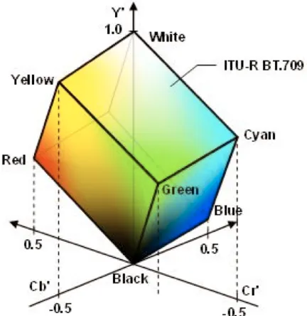
Figure 3.14. Gamut areas of sRGB, YCC and their newly developed, wide-gamut color space, xvYCC [Matsumoto et al., 2006].
In Figure 3.14, a two-dimensional projection of the three-dimensional sRGB gamut is represented, where sRGB values ranging from zero to one are represented on the luma, chroma axes as 0 through 1, -0.5 through 0.5 respectively. These values are also represented as counts 1 through 254, to encompass a digital encoding axis. The color gamut areas corresponding to each color space, shown in Figure 3.14, illustrate the point made about “out-of-gamut” colors. Since the luma component ranges from zero to one, and the chrominance component ranges from -0.5 to 0.5, some unrealizable RGB colors can be represented in terms of YCC coordinates.
and in the conversion back to sRGB, these out-of-gamut colors can theoretically be processed such that clipping is avoided [Sugiura et al.; 2007]. When transforming 8-bit linearized RGB values to YCC space, the range of data values changes.
As shown in Figure 3.14, when converting to YCC, the chroma axis extends from -0.5 to +0.5. As a result, the RGB cube of data points represents only a portion of the YCC space. However, in YCC space, these values are also termed “invalid” since any region outside of the cube cannot be represented in RGB space. This region of YCC encoded colors provides a great opportunity, should an extended display color space become prevalent. Through processing, every RGB color can be converted to achromatic and chromatic signals, where the input YCC values are color managed to the appropriate hue depending on the existence of a negative sign for that particular value. Therefore, colors can be correctly separated and matrixed to corresponding RGB display digital counts when displayed.
Both YCC and sYCC have larger gamuts than sRGB, however, both are also dependent on the output display gamut. Therefore, if the output display gamut is sRGB, the extended gamut areas are limited to the gamut area of sRGB [Kerr; 2005], and thus, will not affect the output colors. Hence, the need for an extended-gamut color space applicable to monitors becomes imperative to successfully display colors outside the sRGB gamut.
3.3.2.3. The premise of YCC
to the CIE definition of L* under CIELAB, and thus, the term luma is used to directly correspond to the digital video signal [Poynton; 2003].
Although not a complete color space, YCC translates digital count information, where the available colorants determine the color displayed. The luma component is computed in Eqn. 3.6,
!
Y'=Kr*R'+(1"Kr"Kb) *G'+Kb*B', (3.6)
where constants Kr and Kb are determined based on the applicable color space. Both constants change depending on the definition of the television (HDTV versus SDTV). The chrominance components equal
!
Pb =1 2*
B'"Y' 1"Kb
Pr =1 2*
R'"Y' 1"Kr
, (3.7) & (3.8)
where the result of Eqns. 3.7 and 3.8 (either Cb/Cr or PbPr) depend on constants Kr and
Kb. R’,G’,B’ are obtained through the opto-electronic transfer function (OETFs)
converting from RGB values. The following equations represent the transfer function incorporated into the conversion. For R,G,B less than or equal to -0.018, Eqn. 3.9 is used.
!
R'="1.099("R)0.45
+0.099 G'="1.099("G)0.45+0.099 B'="1.099("B)0.45
+0.099
(3.9)
If R,G,B is less than 0.018, but greater than -0.018, a scaling factor of 4.50 is applied (Eqn. 3.10).
R'=4.50R
The last case, when R,G,B is greater than or equal to 0.018, Eqn. 3.11 is used.
!
R'=1.099R0.45"0.099
G'=1.099G0.45
"0.099
B'=1.099B0.45"0.099
(3.11)
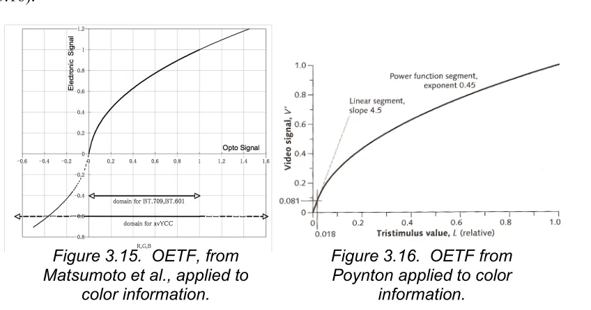
Eqns. (3.8) through (3.10) were explained by both Matsumoto et al., 2006, and Poynton, 2003, in more depth, although differed slightly for cases where R,G,B is less than or equal to -0.018. In Figure 3.15, Matsumoto et al., 2006, considers the negative R,G,B values, whereas Poynton addresses only R,G,B, values between zero and one (Figure 3.16).
[image:53.612.93.517.287.510.2]In both figures, an OETF applied to color information results in the YCC encoded information. Through additional conversions, digital counts can be recovered, as they are for sRGB space, through YCC decoding followed by a transformation corresponding to the Extended ITU-R BT.709-5 and the appropriate color space conversion [Matsumoto; 2006].
Figure 3.15. OETF, from Matsumoto et al., applied to
color information.
Figure 3.16. OETF from Poynton applied to color
3.3.2.4. ITU Existing Standards
The International Telecommunications Union (ITU) is responsible for standardizing specific broadcast signals. ITU-R BT.709.5 is the current standard for YCC encoding on HDTVs, and ITU-R BT.601.5 represents the standard set for SDTV YCC encoding. For short, further reference to the above standards will be denoted as Rec. 709 and Rec. 601. Under both standards, YCC encoding concludes with a matrix transformation converting R’,G’,B’ to Y’CrCb. The matrix, however, varies between Rec. 601 and Rec. 709 as follows:
!
Y'601 Cb'601 Cr'601 " # $ $ $ % & ' ' ' =
0.2990 0.5870 0.1140
(0.1687 (0.3313 0.5000 0.5000 (0.4187 (0.0813
" # $ $ $ % & ' ' ' R' G' B' " # $ $ $ % & ' ' ' (3.12) !
Y'709 Cb'709 Cr'709 " # $ $ $ % & ' ' ' =
0.2126 0.7152 0.0722
(0.1146 (0.3854 0.5000 0.5000 (0.4542 (0.0458
" # $ $ $ % & ' ' ' R' G' B' " # $ $ $ % & ' ' ' (3.13)
When YCC decoding, the inverse OETFs are used in combination with a color space conversion to obtain digital counts corresponding to the appropriate display.
3.3.3. Expanded Gamut Color Space (xvYCC)
The sRGB color space is convenient for displaying images accurately on a display (provided the display has sRGB primaries), without additional consideration of the individual display characteristics [Zeng; 2005]. However, with the addition of more recent technology in expanded gamut displays, sRGB color space may be accurate, but not ideal. Both YCC and sYCC are limited by the output display gamut, and therefore, limit the output values as significantly as sRGB does. Zeng addresses the effect of limiting the number of encoded color amounts. Displaying digital media on a larger gamut, a characteristic of many current displays, and encoding the color information with a smaller color space can result in noticeable quantization errors [Zeng; 2005]. Therefore, research has continued with the rising trend in more colorful displays and a corresponding, expanded gamut color space was sought out.
Displaying colors under conventional sRGB gamut standards on wide-gamut display technology cancels out the attractive characteristics the display holds. Therefore, a new standard wide-gamut color space was proposed as a means to present images on these emerging displays. The color space, xvYCC, was defined by the IEC in 2005, published in January 2006, and investigated by Matsumoto et al. in June 2006.
3.3.3.1. Gamut Area of xvYCC
with reasonable reproduction. Therefore, when converting from sRGB to xvYCC, the gamut area is inherently expanded, and more saturated colors can be represented [Kim; 2007].
This color space was defined for flat panel displays (IEC 2006), as their existence had become quite prevalent, however, their capabilities were not yet used in their entirety. The YCC color space had only begun to approach the desire for extended output gamuts. The cube of encoded YCC colors, from Suriura et al., is displayed in Figure 3.17.
Both “legal” and “illegal” colors are represented in Figure 3.17, according to the
[image:56.612.198.414.300.522.2]definition of the YCC color space [Kim; 2007]. The projections of red, green, blue and white onto the chrominance scale of YCC are represented by the dotted lines. Because Rec. 709 ranges in digital values between zero and one, only the inside cross-section of
Figure 3.17. The cube of encoded colors that comprise the color space defined by
the cube is displayed on Figure 3.17, and on a second reproduction of the figure, Figure 3.18. However, YCC theoretically encompasses both negative R,G,B values and values greater than one (denoted as “invalid” colors earlier).
The footroom and headroom spaces, created by the unused digital counts in the extreme regions, are labeled in Figure 3.18. When converting to xvYCC and extending the digital count ranges to span between one and 254, in both the luma and chroma axes, encoding of a greater number of colors is enabled. This extension is a result of the OETF corresponding to xvYCC, such that the transfer function extends the rhombus in Figure 3.18 to incorporate negative values and values greater than one [Kim; 2007]. These
Figure 3.18. The two-dimensional representation of both the space defined by
![Figure 3.4. Red, Green and Blue LEDs [P.Namek, Wikipedia, 2008]](https://thumb-us.123doks.com/thumbv2/123dok_us/116250.11224/37.612.223.390.71.194/figure-red-green-and-blue-leds-namek-wikipedia.webp)