Decision field theory: Improvements to current methodology and comparisons with standard choice modelling techniques

(1)

This is a repository copy of Decision field theory: Improvements to current methodology and comparisons with standard choice modelling techniques.

White Rose Research Online URL for this paper: http://eprints.whiterose.ac.uk/124426/

Version: Accepted Version

Article:

Hancock, TO, Hess, S and Choudhury, CF orcid.org/0000-0002-8886-8976 (2018) Decision field theory: Improvements to current methodology and comparisons with standard choice modelling techniques. Transportation Research Part B: Methodological, 107 (January 2018). pp. 18-40. ISSN 0191-2615

https://doi.org/10.1016/j.trb.2017.11.004

[email protected] https://eprints.whiterose.ac.uk/ Reuse

Items deposited in White Rose Research Online are protected by copyright, with all rights reserved unless indicated otherwise. They may be downloaded and/or printed for private study, or other acts as permitted by national copyright laws. The publisher or other rights holders may allow further reproduction and re-use of the full text version. This is indicated by the licence information on the White Rose Research Online record for the item.

Takedown

If you consider content in White Rose Research Online to be in breach of UK law, please notify us by

(2)

Thomas O. Hancock (Corresponding Author)

Institute for Transport Studies & Choice Modelling Centre University of Leeds

34-40 University Road Leeds

LS2 9JT

United Kingdom [email protected]

Stephane Hess

[email protected]

Charisma F. Choudhury

(3)

Hancock, Hess and Choudhury 1

ABSTRACT

There is a growing interest in the travel behaviour modelling community in using alternative meth-ods to capture the behavioural mechanisms that drive our transport choices. The traditional method has been Random Utility Maximisation (RUM) and recent interest has focussed on Random Re-gret Minimisation (RRM), but there are many other possibilities. Decision Field Theory (DFT), a dynamic model popular in mathematical psychology, has recently been put forward as a rival to RUM but has not yet been investigated in detail or compared against other competing models like RRM. This paper considers arguments in favour of using DFT, reviews how it has been used in transport literature so far and provides theoretical improvements to further the mechanisms behind DFT to better represent general decision making. In particular, we demonstrate how the probability of alternatives can be calculated after any number of timesteps in a DFT model. We then look at how to best operationalise DFT using simulated datasets, finding that it can cope with underlying preferences towards alternatives, can include socio-demographic variables and that it performs best when standard score normalisation is applied to the alternative attribute levels. We also present a detailed comparison of DFT and Multinomial Logit (MNL) models using stated preference route choice datasets and find that DFT achieves significantly better fit in estimation as well as forecast-ing. We also find that our theoretical improvement provides DFT with much greater flexibility and that there are numerous approaches that can be adopted to incorporate heterogeneity within a DFT model. In particular, random parameters vastly improve the model fit.

KEYWORDS

(4)

1 AN INTRODUCTION TO DECISION FIELD THEORY

Random Utility Maximisation (RUM) models have dominated the field of choice modelling for over 40 years [McFadden, 2000], particularly in travel behaviour research [Ben-Akiva and Bier-laire, 1999]. Recently, however, there has been increasing interest in using alternative methods to make the models flexible to accommodate departures from behaviours assumed under RUM. A key example in transport research has been Random Regret Minimisation [Chorus et al., 2008, Chorus, 2010], which assumes that decision-makers seek to minimise negative emotions rather than max-imising positive ones. Another example comes in the form of Bayesian Belief Networks [Parvaneh et al., 2012], which take a more heuristic approach, looking at an individual’s past experiences and expectations about the different alternatives available.

Whilst these new methods both make more of an effort to consider the underlying cognitive pro-cesses in decision making, another model, Decision Field Theory [Busemeyer and Townsend, 1992, 1993], was designed purely as a cognitive model to capture the deliberation process in deci-sion making. Decideci-sion Field Theory (DFT) is a stochastic-dynamic model of decideci-sion-making be-haviour, which was expanded to include multi-attribute [Diederich, 1997] and then multi-alternative decision-making [Roe et al., 2001], where it was renamed multi-alternative decision field theory (MDFT)1_.

Due to the psychological roots of DFT [Busemeyer and Diederich, 2002], it has predominantly been used to explain behaviour not typically studied using "traditional" choice models. DFT can theoretically explain similarity, attraction and compromise effects [Roe et al., 2001] and this has largely been the focus of DFT research with many papers looking into how well it can explain these context effects compared to other models [Tsetsos et al., 2010, Trueblood et al., 2013, Noguchi and Stewart, 2014]. It is of course true that RUM models can also be used to test such effects, with notably Nested Logit being used to study the similarity effect [Guevara and Fukushi, 2016] or pref-erence reversals [Batley and Hess, 2016]. However, Decision Field Theory further differentiates from these models by being a dynamic model. This means that it can successfully be used to study risky choices or the effect of time pressure [Busemeyer and Townsend, 1993, Diederich, 1997, Dror et al., 1999]. Despite the success of DFT in explaining time and context effects, it has not often been used to explain riskless choices or decision making in general.

We address this research gap in this paper by providing theoretical improvements to further the mechanisms behind DFT to better represent general decision making, incorporating potential ef-fects of socio-demographic variables and accommodating for heterogeneity. The models are rigor-ously compared against RUM and RRM, both for estimation and prediction, using simulated and real datasets.

The remainder of this paper is organised as follows. The next section provides a comprehensive review of DFT: how it works, comparisons with other models and arguments in favour of using DFT. Section 3 gives our theoretical improvements for DFT. Section 4 presents the data and looks at our results from using DFT and section 5 presents some conclusions.

(5)

2 OVERVIEW OF DECISION FIELD THEORY

Thus far, Berkowitsch et al. [2014] have provided the only comparison of DFT against mainstream choice models. As far as we are aware, DFT has never been compared to RRM or other alternative models from choice modelling, nor have the predictive capabilities of DFT been tested. We do not yet know if specific types of choices will be better explained by DFT or if certain decision-makers may be better represented by a DFT model.

In the following subsection, a summary is provided for the basic mechanisms of DFT. We then consider arguments in support of DFT and look further into how it has been used so far in transport research. We conclude by looking at how DFT has been compared to RUM thus far.

2.1 Mechanisms of Decision Field Theory

Basic mechanism

The main idea behind Decision Field Theory is that each available alternative has a ‘preference value’, which updates over time. At each step, the current values are multiplied by a ‘feedback matrix’ before then adding on a valence vector (which can be considered as a utility at a specific moment) at that time. In its most basic form, we have:

Pt =S·Pt−1+Vt, (1)

wherePt is a column matrix containing the current preference values for each alternative at time t, and S is a feedback matrix which contains three parameters (see section 2.1). Pt−1is the previous preference vector and P0 is the initial preference vector. This is often assumed to be [0, ..,0]′

[Busemeyer and Diederich, 2002]. Finally,Vt is the random valence vector at time t, given by:

Vt=C·M·Wt+εt, (2)

whereC is a contrast matrix, used to compare alternatives against each other, with ci,i=1 and

ci,j6=i=−1/(n−1), wherenis the number of alternatives, andM is the attribute matrix. DFT is scale-variant [Busemeyer and Diederich, 2002] and we explore the implications of failing to ensure that the attribute matrix has been appropriately scaled in section 4.3. At each time, t, one attribute is attended to, such thatWt = [0..1..0]′ with entry j=1 if and only if attribute j is the attribute currently being attended to. The probability of attending to attribute j iswj. Since these weights must sum to one, a standard uniform distributionX ∼U(0,1)can be used to select which attribute

a decision-maker attends to at each timestep. It is assumed that there is no relationship between the timesteps, which means an attribute could be considered for several consecutive timesteps before the decision-maker considers a different attribute. There is also a random error vector,εt = [ε..ε]′,

with ε∼N(0,s)added on to allow for flexibility in the variation of probability values that DFT predicts. The variance for the error,s, is often fixed to 1 [Trueblood et al., 2014] but can also be an

estimated parameter.

Calculating expected values

(6)

P1=S·P0+V1 (3a)

P2=S·(S·P0+V1) +V2=S2·P0+S·V1+V2 (3b)

... (3c)

Pt= t−1

∑

k=0

Sk·Vt−k+St·P0 (4)

The weight vectorswjare stationary, thereforeWtcan be considered a stationary stochastic process. This means thatVt is also a stationary stochastic process with meanE[Vt]and a covariance matrix given byCov[Vt]. GivenX, a random vector, andA, a matrix of constants, we have:

var(A·X) =A·var(X)·A′ (5)

We can now use this to calculate the expected valence. We have E[Vt] =µ =C·M·wm, where

wm= [w1,w2, ...,wa]′,andCov[Vt] =Φ=C·M·Ψ·M′·C′+s, whereΨ=Cov[Wt]ands=Cov[εt]. We can then calculate the expected value and covariance of Pt. With S being a constant, E[Pt] reduces to:

E[Pt] =ξt= t−1

∑

k=0

Sk·µ+St·P0 (6a)

= (I−S)−1(I−St)·µ+St·P0 (6b)

Equation 5 also means that we now have:

Cov[Pt] =Ωt=Cov "

t−1

∑

k=0

Sk·Vt−k+St·P0 #

(7a)

=

t−1

∑

k=0

h

Sk·Φ·Sk′i (7b)

The feedback matrix

The feedback matrix is fundamental to the performance of DFT and is defined as:

S=I−φ2×exp(−φ1×D2) (8)

WhereIis an identity matrix,φ1andφ2are sensitivity and memory parameters respectively, andD

is some measure of distance between the attributes across alternatives. The sensitivity parameter, φ1, affects how much alternatives compete with each other. This allows for the similarity effect

to occur [Roe et al., 2001]. The memory parameter, φ2, affects the diagonal entries of the

(7)

different working memory capacities [Daneman and Carpenter, 1980] and memories can grow as well as fade [Mather, 2006], an idea that appears in studies on the validity of eyewitness testimony [Flin et al., 1992, Christianson, 1992, Zaragoza and Lane, 1994]. A number of different methods have been used for defining the distance,D, between alternatives in applications of DFT. Roe et al.

[2001] have suggested that ‘psychological’ distances should be used but in application chose dis-tances that took into account the relative position of the alternatives in the multi-attribute evaluation space. The Euclidean distance (the straight-line distance in the multi-attribute evaluation space) has also been used [Qin et al., 2013]. Psychological distances can be used by including a new third parameter within the feedback matrix, w, so that distances between less competitive alternatives

increase more slowly, as the Euclidean distance fails to account for the fact that some alternative attributes are more important than others [Hotaling et al., 2010]. Berkowitsch et al. [2015] build on this work by creating a generalised distance function for three or more attributes.

Calculating probabilities

Roe et al. [2001] demonstrate that once we have results for the expected value and the covariance of preference values at timet (ξtandΩ_t), we can calculate the probability of choosing alternatives.

They show that on the basis of the multivariate central limit theorem, Pt converges to the multi-variate normal distribution. Under decision field theory,Ais chosen from a set {A,B,C} if it has a

higher preference value at timetthanBandC. It can therefore be calculated as

Pr[Pt[A]−Pt[B]>0∩Pt[A]−Pt[C]>0] =

Z

X>0exp

−(X−Γ)′Λ−1(X−Γ)/2

/(2π|Λ|0.5)dX

(9) withX = [Pt[A]−Pt[B],Pt[A]−Pt[C]]′,Γ=Lξt,Λ=LΩtL′and

L=

1 −1 0

1 0 −1

(10)

Lis a matrix comprised of a column vector of 1s and a negative identity matrix of sizen−1 where nis the number of attributes. The column vector of 1s is placed in the ith column where i is the

chosen alternative. We can then use (for example) the pmnorm package in R [Genz, 1992] to calculate the probability of each alternative being chosen.

Simplifying the deliberation stopping process

The ‘computationally dissatisfying’ process of summing over powers of S (equation 7) can be

avoided by assuming thatt →∞[Berkowitsch et al., 2014]. Therefore, as long as the eigenvalues

ofSare less than one,St→∞. This reduces equation 6 to:

ξ∞= (I−S)−1·µ (11)

More importantly, however, is the simplified form ofΩ_t. From Appendix B of Berkowitsch et al.

[2014], we have:

(8)

Where Φ indicates that Φ has been transformed to a 1×n2 column vector and Z is a n2×n2

matrix based on S. This means that the laborious time-consuming summation in equation 7 can be avoided, but at the cost of assuming that all decision-makers take infinite response time to make their choices.

2.2 Arguments in favour of Decision Field Theory

There are numerous arguments in favour of using DFT. One of the main strength of DFT is that it is a dynamic model, where each alternative has a ‘preference value’, which fluctuates stochastically over time. This means that DFT can explain phenomena such as preference reversal [Diederich, 1997], something that static models, such as most RUM models, cannot do.

DFT is a flexible model, with two methods for a decision-maker to come to a conclusion. The decision-makers can stop deliberating either when they reach an internal threshold value for one of the alternatives or when they reach some external factor, such as a response time limit. This is a parallel to ’satisficing’ behaviour [Simon, 1957] versus maximising behaviour, a concept that was explored by Schwartz et al. [2002]. Some individuals show satisficing behaviour, meaning they choose one of the alternatives when it is good enough (DFT’s internal threshold), whereas others use the full time available to them to try and choose the best alternative, making a decision only when they have to (DFT’s external threshold). Krosnick et al. [1996] demonstrated that satisficing behaviour can often occur when participants complete surveys and Wierzbicki [1982] provides one of the first models incorporating satisficing behaviour.

It has also been demonstrated that context effects, which DFT predicts efficiently, may be fun-damental to decision making [Trueblood et al., 2013], with similarity, attraction and compromise effects all appearing in a perceptual decision task. Whilst there has not yet been a large impact from neuroscience on economics [Krajbich and Dean, 2015], Busemeyer et al. [2006] suggest that the accumulation of preference, as modelled by the behaviourally derived diffusion models in DFT, closely mimics neural activations in non-human primates during perceptual decision-making tasks. For example, Gold and Shadlen [2000] found evidence of an accumulating balance of sensory in-formation favouring one interpretation over another in the neural circuits that generate and inform a monkey’s choice. Ratcliff et al. [2003] similarly found that diffusion models as opposed to Pois-son models better matched the evidence accumulation process seen in neural recordings. Schall [2003] adds that it appears that there are separate neurons initiating responses- a parallel to the threshold value within DFT.

DFT is also less of a ‘black-box’ process than typical RUM models. From a cognitive perspec-tive, basic building blocks of cognition might be shared across a wide range of species and this bottom-top perspective is more in line with both neuroscience and evolutionary biology than the widely used top-down approach [De Waal and Ferrari, 2010]. DFT has a bottom-top perspective, an approach that some researchers believe to be fundamental to understanding individual’s choices if we are to truly understand the underlying cognitive processes in decision making [Otter et al., 2008].

(9)

of alternatives on single dimensions. This would suggest that DFT is an appropriate model when there are two alternatives available, although empirical confirmations for multinomial alternatives are yet to be explored.

2.3 Transport applications of Decision Field Theory

The number of applications of DFT in transport thus far are limited and mainly theoretical. DFT has been suggested as an appropriate mechanism to explain the dynamics and high variability of choice decisions in congestion situations [Stern, 1999], due to its emphasis on an information-processing approach. Additionally, with some expansion, DFT should also be able to deal with a variety of travel situation effects including situational dynamics, type of travel, cultural habits and societal norms [Stern and Richardson, 2005]. The route choice process of a daily commuter according to DFT has been conceptualised [Stern and Portugali, 1999] and DFT has also been combined with the Queuing Network-Model Human Processor to model a driver’s speed control [Zhao et al., 2011]. In an example of actually applying DFT in transport, it was found that given the duration to make a decision, DFT accurately predicted the percentage of participants who chose park and ride, car or bus and subway [Qin et al., 2013]. While these examples demonstrate the potential of DFT in numerous important and relevant applications within transport, they all work with small scale and overly simplified hypothetical studies with limited choice scenarios. Computational limitations of DFT [Otter et al., 2008] have also limited the impact of DFT in the transport literature and there is a distinct research gap in terms of operationalising DFT for full integration in mainstream transport models. For instance, the DFT models tested so far do not account for differences in socio-demographics of the decision-makers, which have been found to have significant effects on RUM and RRM frameworks.

2.4 Decision Field Theory vs Traditional Choice Models

In the only full comparison of DFT with RUM thus far, DFT performed as well as MNL and Probit at predicting consumer product choices made by participants [Berkowitsch et al., 2014]. Additionally, when eliciting context effects, an occurrence of multiple context effects within single participants was found and DFT then performed better than both MNL and Probit, in part due to it being built to cope with such effects. As far as the authors are aware, DFT has never been empirically tested against RRM.

A simplified description of how a DFT model works would be to compare it directly against a MNL or RRM model. Attributes of alternatives,M, are multiplied byW, the relative importance

of the different attributes, which are equivalent to the β coefficients of MNL and RRM. We then getV, a valence vector, which can be considered as ’utility at a specific moment’ and P, the total

preference of alternatives vector, which is equivalent to the utility of alternatives in MNL and total regret in RRM. Whilst DFT models do not produce utilities, we can instead use the total preference of alternatives to calculate the likelihood of alternatives (see equation 4 and section 2.1). Additionally,φ1, the sensitivity parameter, allows for the similarity effect to happen under a

(10)

[image:10.612.75.541.133.278.2]

connectionist interpretation of DFT [Roe et al., 2001]. This demonstrates graphically how the total preference of alternatives is calculated (see equations 1 and 2 for mathematical details).

FIGURE 1: A connectionist interpretation of DFT, adapted from Roe et al. [2001]

2.5 Summary of key DFT applications thus far

Thus far, there have not been many studies that have actually applied Decision Field Theory (par-ticularly within transport). Table 1 provides a summary of some key DFT applications, and high-lights the major differences. Only one major application has been published in a transportation journal until now, with most in psychological journals such as Psychological Review. Whereas some applications only use DFT to calculate the probability of alternatives, there are others that fit choice data to calculate the likelihood of multiple choices, as typically done in a choice modelling study. Very few applications estimate all parameters, with some often held constant. Decision field theory has been applied across a variety of types of choices, most often consumer choice, but also decision making in basketball. Most applications fix the number of timesteps, as prior to this paper, there was no closed form expression for calculating the probabilities of more than three alternatives at any timestep (see section 3.1). When only two alternatives are considered, the number of timesteps does not need to be estimated as Busemeyer et al. [2006] demonstrates that the probability of alternatives can be calculated by instead estimating an internal threshold.

(11)

Hancock,

Hess

and

Choudhury

[image:11.612.77.741.53.598.2]

9

TABLE 1: Some key DFT applications

Authors Journal Type of

estimation

Parameters Type of choices

Key assumptions Key DFT results

Roe et al. (2001) Psychological Review Probability of alternatives Some estimated, some fixed

- - Demonstrated how DFT

explains context effects

Raab and Johnson (2004) Research Quarterly for Exercise and Sport Probability of alternatives Some estimated, some fixed Basketball decisions

- Different initial

preferences explained individual choices best

Scheibehenne et al. (2009)

Cognitive Science

Likelihood of multiple choices,

by individual

All estimated Monetary gambles

Two alternatives, so a timestep parameter

is not required

DFT performs better than the proportional difference model

Tsetsos et al. (2010) Psychological Review Probability of alternatives Some estimated, some fixed

- Used steady

preference states after a large number

of timesteps

DFT performs less well than LCA at explaining

context effects Hotaling et al. (2010) Psychological Review Probability of alternatives Some estimated, some fixed

- - DFT obtains more robust

predictions with internal stopping rules

Hey et al. (2010) Journal of Risk and Uncertainty Likelihood of multiple choices, by individual

All estimated Monetary gambles

Two alternatives, so a timestep parameter

is not required

DFT predicts risky choice better than most other

models considered

Qin et al. (2013) Transportation Research Part F Probability of alternatives Some based on questionnaire Mode choice Feedback coefficients not estimated

Simulated DFT results match survey results

Trueblood et al. (2014) Psychological Review Likelihood of multiple choices across decision makers Some estimated, some fixed Likely crime suspects

1001 timesteps DFT performs less well than MLBA at explaining

context effects

Berkowitsch et al. (2014)

Journal of Experimental Psychology Likelihood of multiple choices across decision makers

All estimated Consumer decisions

Infinite time steps DFT performs as well as MNL and Probit

Noguchi and Stewart

(2014)

Cognition Probability of alternatives Some estimated, some fixed Consumer decisions

1000 timesteps Eye-tracking suggests alternatives are compared

(12)

3 IMPROVEMENTS TO DECISION FIELD THEORY

The following section provides a method for avoiding the sacrifice by Berkowitsch et al. [2014] whilst simultaneously avoiding computationally intensive simulations. We then present methods for incorporating heterogeneity across and within decision-makers into Decision Field Theory.

3.1 Avoiding the sacrifice of response time being set to infinity

It has been argued that the lack of analytical solutions for DFT means that it has to use computa-tionally intensive simulations [Otter et al., 2008] and should be used with an externally controlled stopping procedure with a large value for response time [Trueblood et al., 2014, Noguchi and Stew-art, 2014]. However, Hotaling et al. [2010] argued that the undesirably long fixed stopping times used by Tsetsos et al. [2010] was in part why their DFT model performed worse than their own rival preference accumulation model, the Leaky Competing Accumulator (a model designed to address challenges to previous diffusion, random walk and accumulator models), suggesting that large values for response time should be avoided if possible.

Berkowitsch et al. [2014] avoided arbitrarily setting the number of timesteps by fixing it to infinity, as shown in the previous section. We will now, however, show that as well as being an undesirable sacrifice, this is an unnecessary one. Firstly, we show that the following matrix can be rearranged to a more usable format as follows:

SΦS′=ZΦ (13)

where S is the feedback matrix and Φis the covariance ofVt as before. Again, X indicates that matrixX of sizen×nhas been reshaped into a column matrix of size 1×n2. Now if we start with

any 3 matrices of sizen×n,

A=     

a11 a12 . . . a1n

a21 a22 . . . a2n ... ... ... ...

an1 an2 . . . ann      B=     

b11 b12 . . . b1n

b21 b22 . . . b2n ... ... ... ...

bn1 bn2 . . . bnn      C=     

c11 c12 . . . c1n

c21 c22 . . . c2n ... ... ... ...

cn1 cn2 . . . cnn      (14)

we have that for multiplying matrix A by B, the entry [AB]i j =∑n_k₌1aikbk j. Therefore if we set

ABC=D, we have entries[D]i j=∑nk=1∑nl=1ailblkck j

. Now if we reshape D into a column matrix as before, we haveDwith entries:

D₍_j₋₁₎_n₊_i=

n

∑

k=1

n

∑

l=1

ailblkck j

₍₁₅₎

(13)

Hancock, Hess and Choudhury 11 Z=     

z11 z12 . . . z₁_n2

z21 z22 . . . z2n2 ... ... ... ...

z_n2₁ z_n2₂ . . . z_n2_n2      B=            b11 b21 ...

bn1

b12 ... bnn            (16)

Multiplying these together givesZBwith entriesZB_i=∑n_k₌₁∑n_l₌₁z_i_,₍_k₋₁₎_n₊_lb_lk. This gives us

ZB₍_j₋₁₎_n₊_i=

n

∑

k=1

n

∑

l=1

z₍_j₋₁₎_n₊_i_,₍_k₋₁₎_n₊_lb_lk (17)

Thus forZB=D, we need only setz₍_j−1)n+i,(k−1)n+l =ailck j. Hence we can rearrange equation (13) to this more useful format by settingA=S,B=ΦandC=S′and following the above steps

to find the new matrix Z. We now wish to show that

Sn_Φ_Sn′₌_Zn_Φ ₍₁₈₎

To do this, We employ a proof by induction. We have that equation (18) holds whenn=1 as we know that equation (13) is true. This means that if we can show that equation (19) holds, then we will have proved that equation (18) holds whenn= [2,3,4, ...].

Sn+1_Φ_Sn+1′₌_Zn+1_Φ ₍₁₉₎

Firstly, we set the matricesAn=X,Cn=Y andZn=W. Then the elements of the left side matrix

of equation (19) are:

Now for the right hand side matrix, from the previous result for equation (13) we can set

z₍_j₋₁₎_n₊_i_,₍_k₋₁₎_n₊_l=a_ilc_{k j} (22a)

w₍_j₋₁₎_n₊_i_,₍_k₋₁₎_n₊_l=xilyk j (22b)

and when multiplying these matrices together, we get

so forZW this becomes

ZW B_i=

n

∑

k=1

n

∑

l=1

h

[ZW]_i_,₍_k₋₁₎_n₊_lblk i

(25)

Substituting back in equation (23) and we get

ZW B_i=

n

∑

k=1

n

∑

l=1

" n

∑

r=1

n

∑

s=1

z_i_,₍_s₋₁₎_n₊_rw₍_s₋₁₎_n₊_r_,₍_k₋₁₎_n₊_lblk #

(26)

Finally using equations (22) and rearranging, the right hand side of equation (19) becomes

= [AX BCY]₍_j₋₁₎_n₊_i (27c)

Hence, we have thatZn+1B=An+1_BCn+1_{and the induction is complete. Finally, using this result,}

we can return to equation (7), which now simplifies to become

Cov[Pt] =Ωt= t−1

∑

k=0

h

Sk·Φ·Sk′

i

(28a)

=

t−1

∑

k=0

h

Zk·Φi (28b)

= (I−Z)−1(I−Zt)Φ (28c)

with Z being created from elements of the feedback matrix S by settingz₍_j₋₁₎_n₊_i_,₍_k₋₁₎_n₊_l=silsjk fori,j,k,l∈[1: n]. This means that the time consuming sum calculation has been removed and we

can therefore return to having a finite value fort. We thus restore the original core psychological

foundations of DFT whilst simultaneously avoiding intensive calculations.2

In section 4.2 we compare the results of different versions of DFT, looking at the implications of making this simplification. We compare our version of DFT (DFT-2017), where we estimate the number of timesteps a decision-maker takes to reach a conclusion, against the previous version of DFT (DFT-2014), where decision-makers preferences are assumed to have stabilised over an infinite time. DFT-2014 can be incorporated within DFT-2017, simply by setting the number of timesteps to a high value.

2_{Note that equation 28c becomes equation 12 for}_t_→_∞_{if the eigenvalues of the feedback matrix are less than one}

(15)

3.2 Alternative specific constant (asc) parameters

One of the strengths of RUM models is their ability to measure baseline preferences of some alternatives through the use of alternative specific constants. DFT can partly accommodate this throughP0, the initial preference vector. Crucially, this leads to just an initialpreference for this

alternative, meaning that the preference disappears as the decision time increases and the number of timesteps becomes high. As DFT-2014 has an infinite number of timesteps, this means that it has no method for accommodating initial preferences. However, Roe et al. [2001] used an additional weight assigned to a zero column matrix, as a way of reflecting that the decision-maker was attending to ‘other irrelevant’ attributes (which may actually be relevant). We can expand on this idea by having an additional attribute ‘looking at other factors favouring alternativex.’ This

would have attribute levels ofyfor alternativex, and 0 for all other alternatives. We can either fix yto being a specific value, or allow it to fluctuate by adding it in as another parameter in the same

way that alternative specific constants are. Depending on the number of alternatives, more of these additional attributes can be added as required. This gives us two methods for DFT-2017 and one method for DFT-2014 to deal with preferences towards alternatives, all of which are explored in section 4.3.

3.3 Adding heterogeneity

Decision Field Theory has almost always been implemented as a ‘one size fits all’ model, with an exception being Raab and Johnson [2004], who looked at individual differences in action taking within sport (although this looked at just a single DFT choice scenario, as the attributes were not clearly defined). Scheibehenne et al. [2009] and Hey et al. [2010] also considered individual differences by computing separate DFT models for each decision maker, but as far as we are aware, no studies have thus far fitted a DFT model to multiple decision makers across multiple decisions whilst simultaneously incorporating individual differences. This is surprising given that DFT has psychological origins, where individual differences tend to be better appreciated. Johnson [2006] highlighted the need for DFT to be able to explain individual differences and Liew et al. [2016] found that, as a contradiction to the findings of Berkowitsch et al. [2014], participants rarely showed all three context effects, highlighting the dangers of averaging indiscriminately and not having a method for dealing with individual differences.

(16)

4 EMPIRICAL APPLICATION

4.1 Datasets

In this section we summarise the datasets that we have used to test the explanatory and predic-tive power of Decision Field Theory against other models as well as finding the best methods to maximise the output from a DFT model.

Simulated dataset A (SD-A)

The first simulated dataset contains 1,000 choice situations, each with two attributes ‘A’ and ‘B’, and two alternatives ‘1’ and ‘2’. The attribute values were drawn from a uniform distribution from 1 to 10. After a random number, 0<r< 1, was created for each decision, the probability of

choosing alternative 1 was defined as 0.05WA(A1−A2) +0.05WB(B1−B2) +0.5>r, whereWA andWBwhere the weights of the attributes, both set to 0.5 by default. We use this basic dataset with simple choices to test the ability of a DFT model to capture the effect of underlying preferences for an alternative in section 4.3. A preference for (arbitrarily) alternative 1 is added in by defining that for any choice task with a random number of less than a certain value, the decision-maker would always pick alternative 1.

Simulated dataset B (SD-B)

The second dataset contains 8,000 choice situations, each with six attributes ‘A’ through to ‘F’ and two alternatives ‘1’ and ‘2’. Each attribute value was either true or false. An MNL model was used to simulate the choices (with coefficients βA=−0.6, βB =−0.5, βC =−0.4, βD=−0.3, βE =−0.2 andβF =−0.1). The aim of testing this dataset is to see how well DFT copes with

binary attributes and to compare it against MNL as detailed in section 4.4.

Simulated dataset C (SD-C)

The third dataset also contains 8,000 choice situations, this time with four attributes- cost (TC), travel time (TT), number of changes (CH) and availability of seating (AS). An MNL model was again used to calculate the probabilities of each alternative being picked (with coefficientsβTC = −0.5, βT T =−0.05, βCH =−0.5 and βAS =−0.5). This time a group difference was added in, such that group ‘2’ attached 3 times more value toβAS (for instance, in real life, the decision of some travellers may be strongly affected by the availability of seating). This dataset could then be used to test the ability of DFT to cope with socio-demographic differences as detailed in section 4.5.

Swiss stated preference dataset (SP-1)

(17)

UK stated preference dataset (SP-2)

The second stated preference dataset uses 10 choice tasks from each of 368 participants, all of whom are public transport commuters in the UK. Each task involves an invariant reference trip and two hypothetical alternatives. Each alternative is described by travel time, cost, rate of crowded trips, rate of delays (both out of 10 trips), the average length of delays (across delayed trips) and cost of a provision of a delay information service [Hess and Stathopoulos, 2013].

4.2 Differences between different DFT models

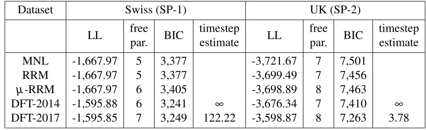
In this section we compare DFT-2014 (DFT without a time parameter) against DFT-2017 (DFT with a time parameter). The DFT model with a time parameter uses the method described in section 3.1 whilst the one without follows the method of Berkowitsch et al. [2014], where response time is set to infinity. We also compare these models against simple multinomial logit models and also two versions of random regret minimisation models (the first following the specification of [Chorus, 2010]) and the second following [van Cranenburgh et al., 2015], incorporating µ, a parameter to estimate a profundity of regret). For SP-1, our MNL and RRM models contain five parameters, four for the attributes and one alternative specific constant. SP-2 has an additional attribute and an additional alternative, resulting in seven parameters. Theµ-RRM models have six and eight parameters respectively with the addition of theµparameter. The DFT models have three and four parameters respectively for attributes in SP-1 and SP-2. All DFT models additionally have sensitivity, memory and error parameters (φ1,φ2 and ε) and DFT-2017 models also have a

[image:17.612.89.519.431.563.2]

parameter for the number of timesteps.

TABLE 2: Results from removing the sacrifice of setting response time to infinity

Dataset Swiss (SP-1) UK (SP-2)

LL free BIC timestep LL free BIC timestep

par. estimate par. estimate

MNL -1,667.97 5 3,377 -3,721.67 7 7,501

RRM -1,667.97 5 3,377 -3,699.49 7 7,456

µ-RRM -1,667.97 6 3,405 -3,698.89 8 7,463

DFT-2014 -1,595.88 6 3,241 ∞ -3,676.34 7 7,410 ∞

DFT-2017 -1,595.85 7 3,249 122.22 -3,598.87 8 7,263 3.78

(18)

Whilst the weight estimates are similar (Table 15), the psychological parameters also have some-what different estimates. However, the minimal impact these parameters have on the preference values (see appendix D) suggests that the difference in goodness of fit is more likely to be a result of the difference in the number of timesteps. For SP-1, DFT has two more parameters than MNL, and it could be argued that BIC values do not penalise this difference enough. However, we find that the best fitting MNL model with an additional two parameters (square root terms for cost and time) has a log-likelihood of−1,615.79, which is still significantly worse than DFT.

4.3 Implementation and application of Decision Field Theory

In this section we look at how to best implement and apply a Decision Field Theory model. We consider the implications of the weight parameters having to be greater than zero, look at methods for DFT to incorporate underlying preferences for an alternative and look at the effect of different scaling methods being used on the attribute levels3_.

Implications of Decision Field Theory weight parameters having to be greater than zero

Using the Swiss stated preference dataset (SP-1), it is quickly possible to see the effect of hav-ing undesirable attributes in DFT. If a value for an undesirable attribute is positive and high (for example, a large cost), then an appropriate DFT model would factor this in by adding a negative valence to the preference value of an alternative when this attribute is considered. However, the weight parameters in a DFT model cannot be negative, aswirepresents the proportion of time that a decision-maker looks at attributei. This causes issues when we have ‘positive’, desirable attributes

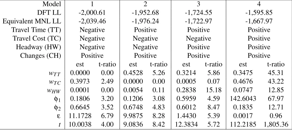
(such as quality), and ‘negative’, undesirable attributes (such as travel cost). If the attributes were to be left as they were, then due to DFT being an accumulative model and weights being positive, there would be no way for DFT to reflect that an alternative is more likely to be picked if an at-tribute level is lower. This means that DFT will have its greatest predictive accuracy when negative attributes are ignored, and their weights are set to zero. Table 3 shows the log-likelihood values of SP-1 under DFT models where some attributes are desirable/undesirable. As all four attributes are undesirable, ’negative’ here means that the higher values are less desirable, whereas positive means that they have been reset such that higher, more positive values are more desirable. The table also shows the parameter estimates for the DFT models. As DFT has no clear starting points for estimation, we have to run a number of trials to find a suitable starting point. We set the weight attributes to be equal and use random numbers to setφ1 between 0 and 10, φ2 between 0 and 1,

ε between 0 and 1,000 andt between 0 and 100. We ran 100 trials of this nature and then used

the best as the starting point in the R package maxLik [Henningsen and Toomet, 2011]. We found that the inclusion of the third feedback parameter,w, made an insignificant difference to the results

of DFT, therefore omitted it in these trials and used Euclidean distances in the feedback matrix. We used standard score normalisation to scale the attributes in this section, but explore scaling methods further in section 4.3.

We can see from Table 3 that if the travel costs are negative (Model 3), the parameter for travel cost,wTC, quickly drops towards zero, reflecting that the DFT model has not used the information as to do so would worsen model fit. An equivalent hindrance on a MNL model, where the beta coefficient for travel cost is fixed to zero, suffers a similar loss in log-likelihood. When headway

(19)

[image:19.612.74.565.111.331.2]

TABLE 3 : Parameter estimates and log-likelihoods for DFT models for positive and negative attributes (using SP-1)

Model 1 2 3 4

DFT LL -2,000.61 -1,952.68 -1,724.55 -1,595.85

Equivalent MNL LL -2,039.46 -1,976.24 -1,722.97 -1,667.97

Travel Time (TT) Negative Positive Positive Positive

Travel Cost (TC) Negative Negative Negative Positive

Headway (HW) Negative Negative Positive Positive

Changes (CH) Positive Positive Positive Positive

est t-ratio est t-ratio est t-ratio est t-ratio

wT T 0.0000 0.00 0.4528 5.26 0.3214 5.86 0.3475 45.31

wTC 0.3973 2.49 0.0000 0.00 0.0005 0.07 0.4676 43.22

wHW 0.0001 0.00 0.0054 0.11 0.2838 15.18 0.0747 12.85

φ1 0.1806 3.20 0.1206 3.08 0.5959 4.59 142.6043 67.97

φ2 0.6645 3.52 0.6748 4.83 0.6012 8.47 0.1835 12.71

ε 11.1728 6.79 9.9875 8.28 1.4430 5.39 0.0017 0.96

t 10.0038 4.00 9.0836 8.42 12.3834 5.72 112.2185 1,805.36

is also negative (model 2),wHW also drops to zero. The value for the error term,ε, has increased significantly. Hotaling et al. [2010] argue that the error term (also known as the noise variance [Roe et al., 2001]) would be higher for more complex tasks, meaning that higher values for ε would be found for less predictable decisions, as demonstrated here. Model 1, where travel time is made negative, obtains further losses in model fit. Perhaps surprisingly, the coefficient for travel cost weight increases away from zero. However, this is due to alternatives with low travel time and high cost being generally preferred to alternatives with high travel time and low cost. This is also reflected in an MNL model with just beta coefficients for travel cost and the number of changes, in which a positive value (βT T =0.015, t-ratio=2.34) for travel cost is found.

The memory parameter, φ2, is higher for models with negative attributes, suggesting that DFT

(20)

Dealing with underlying preferences

Random Utility Models with a Multinomial Logit framework deal with underlying preferences through alternative specific constants [McFadden and Train, 2000]. These values directly capture market shares. DFT has two methods for capturing shares and dealing with preferences towards an alternative. One is through the initial preference matrixP0 and the other is by creating a new

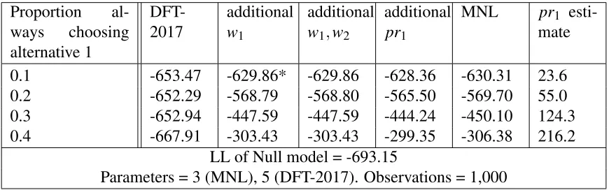
attribute favouring one of the alternatives. Here we simply add in a dummy variable for the al-ternatives with a higher value for one of the alal-ternatives. Table 4 displays the results of adding in additional DFT parameters to deal with preferences in simulated dataset A. A parameter pr1

indicates an initial preference for alternative 1 in P0 and parametersw1,w2 indicate weights for

[image:20.612.89.524.261.397.2]

new attributes favouring alternative 1 and 2 respectively.

TABLE 4: The effect of underlying alternative preferences on DFT models (using SD-A)

Proportion al-ways choosing alternative 1

DFT-2017

additional

w1

additional

w1,w2

additional

pr1

MNL pr1

esti-mate

0.1 -653.47 -629.86* -629.86 -628.36 -630.31 23.6

0.2 -652.29 -568.79 -568.80 -565.50 -569.70 55.0

0.3 -652.94 -447.59 -447.59 -444.24 -450.10 124.3

0.4 -667.91 -303.43 -303.43 -299.35 -306.38 216.2

LL of Null model = -693.15

Parameters = 3 (MNL), 5 (DFT-2017). Observations = 1,000

For the models in Table 4, we set the attribute value difference for the new parameterw1to 5

arbi-trarily in every case. A value of−629.99 was achieved in case * when a value of 1 is used instead.

This value could be set as another parameter, but as the value has not changed significantly we have not explored this further.

Whereas adding in parameter w1 for a preference of alternative 1 makes a difference, the weight

for the preference of alternative 2,w2, drops to 0. This means that we can treat these parameters

equivalently to alternative specific constants in random utility models, where similarly only one parameter would be needed to capture the difference in underlying preferences between two alter-natives. We can see from Table 4 that adding inw1results in DFT achieving similar LL values to

MNL. However, better values are achieved by adding in the parameter pr1. As the percentage of

choices where decision-makers always choose alternative 1 increases, the parameter estimate for

pr1rises, as does the difference between MNL and DFT LL values.

Using DFT-2014, where the number of timesteps is set to infinity, results in only a few differ-ences for this dataset. This is because the estimate for the number of timesteps is high (see Table 3). Without additional weights, the same log-likelihood values are achieved. However, with one additional weight parameter, the log-likelihood is−447.78 when the proportion always choosing

alternative 1 is 0.3, slightly lower than the log-likelihood achieved for DFT-2017. This difference results from the parameter estimate for φ2, the memory parameter, being negative for this model

(−0.0004). The estimate forφ2cannot be negative under a version of DFT where the number of

(21)

resulting in a preference matrix that never converges.

Scaling of attributes

The most common method for scaling attributes that has been used in previous applications of DFT has been to rescale values to be between two values (unity-based normalisation) [Berkowitsch et al., 2014, Johnson, 2006]. We now consider different methods for scaling the attribute values in dataset SP-1 and the effects this has on the parameter estimates for DFT. The first method we use is unity-based normalisation, where we have a minimum value of 0 and maximum value of 1. We setai=1−_maxai₍−_a₎min₋_min(a)₍_a₎ for each of the attributes, ensuring that we set the most desirable attribute level (lower costs and travel times) to be close to 1 and less desirable attribute levels to be close to 0. For the second method, we do not scale the attributes at all, simply settingai=−ai. For the third method, we use standard score normalisation and set ai=−ai−_sdmean₍_a₎(a). The fourth method employs the same values as the third, with the exception that the travel time values are additionally all multiplied by 10.

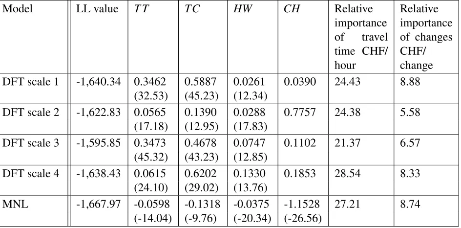
Table 5 shows the weight estimates for each attribute in the different DFT models as well as the MNL beta coefficient values for travel time (TT), travel cost (TC), headway (HW) and the number of changes made when travelling by train (CH). As with other departures from RUM, value of time and similar measures cannot be directly calculated under a DFT model. We instead define ‘relative importance of time,’ as wT T/ST T

[image:21.612.76.548.445.678.2]

wTC/STC ×60, whereSi is the scale factor used for scaling attributei, and use the value of time for the relative importance of time under MNL.

TABLE 5 : Parameter estimates (t-ratios in brackets) for DFT models under different types of scaling for SP-1

Model LL value T T TC HW CH Relative

importance of travel time CHF/ hour

Relative importance of changes CHF/ change

DFT scale 1 -1,640.34 0.3462 0.5887 0.0261 0.0390 24.43 8.88

(32.53) (45.23) (12.34)

DFT scale 2 -1,622.83 0.0565 0.1390 0.0288 0.7757 24.38 5.58

(17.18) (12.95) (17.83)

DFT scale 3 -1,595.85 0.3473 0.4678 0.0747 0.1102 21.37 6.57

(45.32) (43.23) (12.85)

DFT scale 4 -1,638.43 0.0615 0.6202 0.1330 0.1853 28.54 8.33

(24.10) (29.02) (13.76)

MNL -1,667.97 -0.0598 -0.1318 -0.0375 -1.1528 27.21 8.74

(-14.04) (-9.76) (-20.34) (-26.56)

(22)

It appears that because of the large range of attribute values, some of the information is lost in method 1. The high weight value for the number of changes in scale 2, 0.7767, shows that due to the lack of scaling, the decision-maker has to attend to the number of changes more often for the importance of this attribute to be reflected. The best log-likelihood value under DFT is achieved in scale 3, suggesting that it is important to include information on means and standard deviations when scaling the attribute values before running a DFT model. The relative importance of travel time and the relative importance of changes estimates vary depending on which type of scaling is used. It appears that as the model’s log-likelihood value improves, both relative importance values decrease.

Table 5 also shows the impact of multiplying the travel times in SP-1 by 10 in DFT scale 4. The only difference this makes for a RUM Multinomial Logit is that the travel time coefficient becomes exactly 10 times lower. As a contrast, DFT does not equivalently have a simple change of coefficients. Instead, we see that wT T has decreased from 0.3473 to 0.0615. This reflects the fact that to capture the relative importance of time, it has to be attended to less often relative to the other attributes for it to be appropriately incorporated into the model. We see a lower value of log-likelihood, with the increase in relative importance values likely being the cause.

4.4 Differences in results between Decision Field Theory and other models

Exploring the differences between RUM Multinomial Logit and Decision Field Theory probabilities

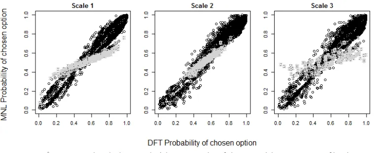
[image:22.612.113.493.470.626.2]

The different scaling methods for the attribute values for a DFT model has a big impact on the dif-ferences between DFT and MNL model probability of alternatives for SP-1. Figure 2 demonstrates that scales 1 and 3 in particular find that when the number of changes and headway is the same for both alternatives, DFT makes a more extreme prediction than MNL, indicated by the grey points on the figure. This does not happen under scale 2, where DFT makes more conservative predictions.

FIGURE 2: Difference between MNL and DFT probabilities of chosen alternatives for SP-1

(23)

but that it decreases as the difference between the number of changes, travel time and headway between the alternatives increases.

This is also the case in simulated datasetA, where similarly, linear regression shows that the

ab-solute difference between MNL and DFT probabilities decreases as the differences between the alternatives increase. Simulated dataset B finds an extremely small average difference between

MNL and DFT of 9.51e−05, with standard deviation 0.0041 and a largest difference of 0.008.

This suggests that if alternatives only have true/false attributes, DFT will produce very similar re-sults to MNL.

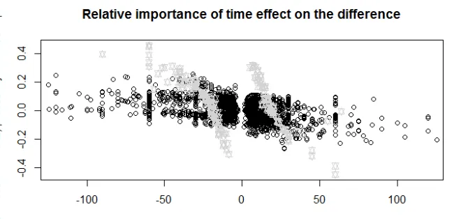
[image:23.612.142.467.306.463.2]

We also have from figure 3 that the relative importance of travel time has a significant impact on the difference between MNL and DFT. The relative importance of travel time of an alternative is defined here as being positive if the more expensive, faster alternative is chosen and negative if the cheaper, slower alternative is chosen. For example, a value of 50 indicates that the decision-maker is spending 50CHF per hour saved.

FIGURE 3: Impact of the relative importance of time on the difference between MNL and DFT probabilities of chosen alternatives for SP-1

From Table 5 we can see that DFT (scale 3) predicts a relative importance of travel time of 21.4 whereas MNL predicts a relative importance of travel time of 27.2. This difference is reflected in figure 3 by the fact that the lower the relative importance of travel time is, the larger the difference between DFT and MNL becomes in favour of DFT. We also see for decisions that are purely a trade-off between time and cost (grey points), the impact of the value of the relative importance of time is larger for DFT.

(24)

[image:24.612.138.451.85.399.2]

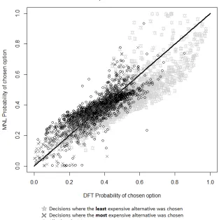
FIGURE 4: Difference between MNL and DFT probabilities of chosen alternatives for SP-2

(25)

[image:25.612.121.502.84.281.2]

FIGURE 5: Difference between MNL and DFT log-likelihoods for individuals

Runtime of Decision Field Theory

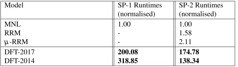
[image:25.612.114.502.434.544.2]

Decision Field Theory is a relatively slow model to run. Table 6 shows the runtimes for datasets SP-1 and SP-2. The runtimes are normalised relative to the runtime for MNL for SP-1 and SP-2.

TABLE 6: Relative runtimes of models for SP-1 and SP-2

Model SP-1 Runtimes SP-2 Runtimes

(normalised) (normalised)

MNL 1.00 1.00

RRM - 1.58

µ-RRM - 2.11

DFT-2017 200.08 174.78

DFT-2014 318.85 138.34

(26)

4.5 Incorporating Heterogeneity

Using socio-demographic variables in Decision Field Theory

One strength of RUM models is that they are good at using the input of socio-demographic vari-ables to improve model accuracy. As far as we are aware, these factors have never been incorpo-rated into DFT. This idea is explored in this section.

Firstly, we explore the impact of income on the weight parameter for travel cost, wTC for SP-1. Whilst attribute parameters for MNL are independent of each other, this is not the case for DFT weight parameters, as together they sum to 1. We hence definewTC =wTC+x, with the other pa-rameters adjusted towi=wi−x×₁₋w_wi_TC, wherexis defined asx=pHI×HI,HI is the household income and pHI is a new parameter defining the strength of the impact of income. For our MNL model, income is included in the utility functions by using pHI×HI×tc, where tcis the travel cost of the alternative. Table 7 shows the results of including the income parameter on each of the standard models.

TABLE 7: Log-likelihood values for models with and without income/group difference parameter (using SP-1 and SD-C)

SP-1 Basic model With income parameter

MNL -1,667.97 -1,653.61

DFT -1,595.85 -1,592.35

SD-C Basic model With group parameter

MNL -4,633.90 -4,509.65

DFT -4,633.63 -4,527.56

Whilst there is some improvement in the result for the DFT model in SP-1, it is not as large as the improvement in the MNL model. This however does not appear to have a significant impact on the differences between MNL and DFT probabilities of chosen alternatives (see figure 6 in appendix C).

We also explore the impact in a deliberately manipulated simulated dataset. Using simulated dataset C, we look at the improvements under MNL and under DFT by including a parameter

to control which group the decision belongs to. As before for DFT, we add a factorxto the weight

for seating/standing, subtracting this amount proportionally from the other weights. We setx=pG for group 1, andx=0 for group 2. For MNL, we add pG×Sonto the utility for both alternatives for group 1, where S is equal to 1 or 0 depending on whether seating is available. Table 7 also

shows the results of including a parameter for this group difference on each of the standard mod-els. Once again, it appears that whilst DFT improves with the inclusion of this socio-demographic variable, MNL improves more significantly.

Adjusting psychological parameters in Decision Field Theory

We can additionally make small changes to the psychological parameters,φ1andφ2, the sensitivity

(27)

adjust the memory parameter depending on how many choice tasks the decision-maker has already completed. We add a new variable, φ3, such that our memory parameter is now φ2+φ3×n,

[image:27.612.127.488.177.244.2]

where n is the task number. Alternatively, the sensitivity parameter can be similarly adjusted to be φ1+φ3×n. Results from both of these adjustments are in Table 8.

TABLE 8 : Log-likelihood values for models with and without adjustments to the memory and sensitivity parameters

Model Swiss (SP-1) UK (SP-2)

DFT -1,595.85 -3,598.87

φ1adjusted -1,595.13 -3,592.15

φ2adjusted -1,595.67 -3,594.78

Whilst the adjustments make very little difference for SP-1, there is a significant effect for SP-2, as only one parameter has been added. This suggests that improving the flexibility of the psycholog-ical parameters has the potential to allow for a changing neurologpsycholog-ical state in the decision-maker.

Adding heterogeneity: Mixed DFT

Our final effort to add heterogeneity to a DFT model is to use random parameters. For both DFT with and without a parameter for the number of timesteps, a significant improvement in fit is found (Table 9). For weight parameters, which cannot be less than zero, we use truncated normal distributions. We trial both normal and truncated normal distributions for the remaining parameters. These are then compared against DFT models with fixed parameters as well as against a DFT model without a time parameter with truncated normal distributions for all parameters. All mixed models are estimated using Dumont et al. [2014]’s R package ’RSGBH’.

TABLE 9: Log-likelihoods of Mixed Decision Field Theory Models

Model Time

parameter?

Weight parameters

Other parameters

Swiss (SP-1) UK (SP-2)

pars LL BIC pars LL BIC

1 yes fixed fixed 7 -1,595.85 3,249 8 -3,598.87 7,263

2 no fixed fixed 6 -1,595.88 3,241 7 -3,676.34 7,410

3 yes truncated normal 14 -1,450.39 3,015 16 -3,156.27 6,444

4 yes truncated truncated 14 -1,438.39 2,991 16 -3,140.09 6,412

5 no truncated truncated 12 -1,430.41 2,959 14 -3,190.23 6,495

For both datasets, vast gains are made by using random parameters. A better fit is found if truncated normal distributions are used for all parameters rather than just the weight parameters. Using random parameters in Berkowitsch et al. [2014]’s version of DFT results in a lower BIC value for the SP-1 but a much higher one for SP-2. Whilst we do not run mixed multinomial logit or mixed random regret models, Hess et al. [2016] do run these models on the same UK dataset (see appendix B for a table of results). They find that their best fitting model is a mixedµ-RRM model, which achieves a log-likelihood of−3,174.96 with a BIC of 6,456.66. Whilst Mixed DFT has a

[image:27.612.70.580.470.581.2]

(28)

4.6 Predictive capabilities of Decision Field Theory

As discussed in section 1, previous researchers have only compared the goodness-of-fit of DFT, and its performance in the context of forecasting has not been tested before. We have looked at the predictive capabilities of DFT on both of our route choice stated preference datasets, SP-1 and SP-2. We adopt the method used by Frejinger and Bierlaire [2007], using 80% of the data drawn randomly 5 times for estimation. These estimates are used to calculate probabilities for different choice outcomes for the remaining 20%, and a choice is then assigned probabilistically. We then obtain likelihoods for the forecasted decisions being observed. The results for SP-1 and SP-2 are displayed in Tables 10 and 11, respectively.

[image:28.612.73.557.416.643.2]

Table 12 shows that the likelihood ratio tests obtained comparing DFT against MNL for SP-1 indi-cate that the DFT model is significantly better for both estimation and forecasting. Whilst DFT is significantly better for forecasting results, the differences are more extreme for estimation results, where DFT produces much higher log-likelihood values. From Table 10 we can see that DFT achieves higher log-likelihood values thanµ-RRM in all estimated and forecasted datasets. Like-lihood ratio tests show that DFT produces significantly better results than MNL and RRM (which both have one less parameter) too for both estimation and forecasting (see Table 13). Whilst RRM achieves results closer to DFT than MNL does, it is still significantly worse than DFT for all datasets. These results suggest that DFT is an appropriate model for both estimation and forecast-ing.

TABLE 10: Log-likelihoods for the estimated and forecasted datasets for MNL and DFT (using SP-1)

Model Swiss (SP-1) Dataset 1 Dataset 2 Dataset 3 Dataset 4 Dataset 5

Estimated Final LL -1,356.52 -1,324.59 -1,338.47 -1,333.51 -1,365.84

80% ρ2 0.298 0.315 0.308 0.310 0.294

MNL Forecasted Final LL -308.25 -319.612 -322.409 -326.311 -342.081

5 parameters 20% ρ2 0.355 0.332 0.326 0.318 0.286

Full Final LL -1,664.77 -1,644.2 -1,660.88 -1,659.82 -1,707.92

100% ρ2 0.312 0.320 0.314 0.314 0.294

80% ρ2 0.324 0.344 0.336 0.344 0.319

DFT Forecasted Final LL -296.068 -294.684 -290.9 -294.191 -327.112

7 parameters 20% ρ2 0.376 0.379 0.387 0.380 0.312

Full Final LL -1,601.64 -1,560.91 -1,572.44 -1,561.16 -1,641.98

(29)

[image:29.612.76.556.202.632.2]

TABLE 11: Log-likelihoods for the estimated and forecasted datasets for MNL, DFT, RRM and µ-RRM (using SP-2)

Model UK (SP-2) Dataset 1 Dataset 2 Dataset 3 Dataset 4 Dataset 5

80% ρ2 0.073 0.079 0.079 0.075 0.087

MNL Forecasted Final LL -761.76 -748.97 -743.77 -752.80 -720.37

7 parameters 20% ρ2 0.049 0.065 0.071 0.060 0.100

Full Final LL -3,754.48 -3,720.06 -3,715.82 -3,739.08 -3,664.81

100% ρ2 0.070 0.078 0.079 0.073 0.092

80% ρ2 0.105 0.109 0.111 0.108 0.108

DFT Forecasted Final LL -704.46 -717.87 -702.70 -704.55 -681.86

8 parameters 20% ρ2 0.119 0.102 0.121 0.119 0.147

Full Final LL -3,592.53 -3,605.89 -3,570.78 -3,581.11 -3,569.88

100% ρ2 0.109 0.106 0.115 0.112 0.115

80% ρ2 0.077 0.083 0.084 0.080 0.093

RRM Forecasted Final LL -754.66 -744.29 -739.96 -747.77 -715.22

7 parameters 20% ρ2 0.058 0.071 0.076 0.067 0.107

Full Final LL -3,731.59 -3,702.57 -3,695.89 -3,717.27 -3,643.23

100% ρ2 0.075 0.082 0.084 0.079 0.097

80% ρ2 0.077 0.083 0.084 0.080 0.092

µ-RRM Forecasted Final LL -753.91 -746.28 -740.83 -750.04 -715.08

8 parameters 20% ρ2 0.058 0.067 0.074 0.062 0.106

Full Final LL -3,730.65 -3,704.56 -3,696.46 -3,719.11 -3,642.96

(30)

[image:30.612.182.430.138.361.2]

TABLE 12: Likelihood Ratio Tests for the estimated and forecasted results of DFT against MNL (using SP-1)

Swiss (SP-1) MNL/DFT

Estimated Forecast

Dataset 1 T-stat 101.90 24.36

p-value 3.7E-23*** 2.6E-10***

p-value 2.3E-26*** 7.5E-12***

Dataset 3 _{p-value 9.4E-26*** 1.0E-14***}T-stat 113.86 63.02

Dataset 4 _{p-value 6.3E-30*** 5.6E-15***}T-stat 133.08 64.24

p-value 3.7E-23*** 1.6E-07*** Signif. codes: ***<0.001 **<0.01 *<0.05 .<0.1

TABLE 13: Likelihood Ratio Tests for the estimated and forecasted results of DFT against MNL and RRM (using SP-2)

UK (SP-2) MNL/DFT RRM/DFT µ-RRM/DFT

Estimated Forecast Estimated Forecast Estimated Forecast

Dataset 1 T-stat 209.39 114.60 177.81 100.40 177.43 98.90

p-value 9.4E-48*** 4.9E-27*** 7.3E-41*** 6.3E-24*** 8.9E-41*** 1.3E-23***

Dataset 2 T-stat 195.34 62.21 169.65 52.84 169.65 56.82

p-value 1.1E-44*** 1.6E-15*** 4.4E-39*** 1.8E-13*** 4.4E-39*** 2.4E-14***

Dataset 3 T-stat 207.92 82.15 175.70 74.52 175.09 76.26

p-value 2.0E-47*** 6.4E-20*** 2.1E-40*** 3.0E-18*** 2.9E-40*** 1.3E-18***

Dataset 4 T-stat 219.45 96.49 185.88 86.44 185.03 90.98

p-value 6.0E-50*** 4.5E-23*** 1.3E-42*** 7.3E-21*** 1.9E-42*** 7.3E-22***

Dataset 5 T-stat 135.51 77.02 102.64 66.73 102.38 66.45

[image:30.612.73.587.469.692.2]