Consensus via multi-population robust mean-field games

This is a repository copy of Consensus via multi-population robust mean-field games. White Rose Research Online URL for this paper:

http://eprints.whiterose.ac.uk/119335/ Version: Accepted Version

Article:

Bauso, D. orcid.org/0000-0001-9713-677X (2017) Consensus via multi-population robust mean-field games. Systems and Control Letters, 107. pp. 76-83. ISSN 0167-6911

https://doi.org/10.1016/j.sysconle.2017.07.010

Article available under the terms of the CC-BY-NC-ND licence (https://creativecommons.org/licenses/by-nc-nd/4.0/)

Reuse

This article is distributed under the terms of the Creative Commons Attribution-NonCommercial-NoDerivs (CC BY-NC-ND) licence. This licence only allows you to download this work and share it with others as long as you credit the authors, but you can’t change the article in any way or use it commercially. More

information and the full terms of the licence here: https://creativecommons.org/licenses/

Takedown

If you consider content in White Rose Research Online to be in breach of UK law, please notify us by

Consensus via multi-population robust mean-field games

D. Bausoa,b

a

Department of Automatic Control and Systems Engineering, The University of Sheffield, Mappin Street, Sheffield, S1 3JD, United Kingdom

b

Dipartimento di Ingegneria Chimica, Gestionale, Informatica, Meccanica, Universit`a di Palermo, V.le delle Scienze, 90128 Palermo, Italy.

Abstract

In less prescriptive environments where individuals are told ‘what to do’ but not ‘how to do’, synchronization can be a byproduct of strategic thinking, prediction, and local interactions. We prove this in the context of multi-population robust mean-field games. The model sheds light on a multi-scale phenomenon involving fast synchronization within the same population and slow inter-cluster oscillation between different populations.

Keywords: Synchronization, Consensus, Mean-field games

1. Introduction

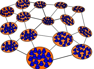
Synchronization is a natural phenomenon which arises in many applica-tions such as pricing in finance [2, 5], opinion dynamics [13], or transient stability of generators [3] etc. Most of the models for synchronization are derived in prescriptive environments in which individuals, the agents, are pre-programmed to adopt specific behaviors, see [12] and references therein. In this paper we consider a multi-population of dynamic agents as illus-trated in Fig. 1.

The dynamics of each agent — henceforth referred to as microscopic dy-namics — describes the time evolution of its state in the form of a stochastic differential equation. In addition, for each population of agents, we consider the corresponding phase coherence, which is a measure of the synchroniza-tion of the agents of that populasynchroniza-tion, and the associated dynamics, the latter called macroscopic dynamics. Each agent seeks to synchronize its phase to

Figure 1: Multi-population model with local interactions.

the local average phase obtained via mean-field computation. The model highlights the following aspects: i) each agent is a rational player equipped with strategic and computation capabilities; ii) the interaction is local and subject to disturbances; iii) agents are heterogeneous. Local interaction is determined by geographic proximity between two populations, and is mod-eled by a network topology where the nodes are the populations and the links establish neighbor relations. The model is a multi-population robust mean-field games within the theory proposed by M.Y. Huang, P. E. Caines and R. Malham´e in [6, 7, 8] and independently by Lasry and Lions in [10]. For a survey see [4]. Modeling synchronization as a game is also in [15]. Game theoretic learning is also discussed in [16]. Efficiency loss in equilibria is studied in [17]. Higher level interactions between the subpopulations are analyzed in [9] in the context of auctions. While sharing some of the general concepts already present in the aforementioned references, this paper adds new elements such as local interactions, disturbances and heterogeneity in a unified framework.

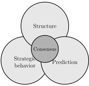
Strategic behavior

Structure

Prediction

Consensus

Figure 2: Synchronization as a result of a proper mix of strategic thinking, prediction, and local interaction in a structured environment.

The model involves a system of coupled partial differential equations (PDEs). For each population we have one PDE in the form of a Hamilton-Jacobi-Isaacs (HJI) equation, and a second PDE which is the Fokker-Planck-Kolmogorov (FPK) equation describing the diffusion process of the agents’ states. We provide a solution of the HJI equation under the assumption that the time evolution of the common state is given. We show that the problem reduces to solving three matrix equations and that in the infinite horizon case the macroscopic dynamics is a typical consensus dynamics.

The analysis of the mean-field game is then extended to the case of second-order dynamics. Even for this case, we prove that the problem of approx-imating mean-field equilibrium strategies reduces to solving three matrix equations. By taking the limit for T → ∞ the macroscopic dynamics takes the form of a second-order consensus dynamics. Simulations of simple heuris-tics show the multi-scale nature of the process involving fast synchronization within the same population and slow inter-cluster oscillation capturing delays due to the geographic sparsity of the populations.

2. Model and problem set-up

Consider ppopulations of homogeneous agents (players); each player be-longs to a populationk ∈ {1, . . . , p}and is characterized by a stateX(t)∈R

at time t∈[0, T], where [0, T] is the time horizon window. The control vari-able is a measurvari-able function of time, u(·) ∈U, where U is the control set, defined as t 7→Rand establishes the rate of variation of an agent’s state. A disturbance tries to affect the agents’ state in a way that is proportional to his efforts w(·)∈W, whereW is the control set of the disturbance.

The state dynamics of each player is

dX(t) = (u(t) +w(t))dt+σdB(t), t >0, (1)

where X(0) =xfor given initial state x,σ >0 is a weighting coefficient and B(t) is the standard Brownian motion process.

For every population k ∈ {1, . . . , p}, consider a probability density func-tion mk : R×[0,+∞[→ R, (x, t) 7→ mk(x, t), representing the density of agents of that population in statexat timet, which satisfies R_Rmk(x, t)dx= 1 for every t. Let the mean state of population k at time t be mk(t) :=

R

Rxmk(x, t)dx. From averaging both sides of (1) we get the aggregated dy-namics

d

dtmk(t) =uk(t) +wk(t),

where uk(t) and wk(t) are the mean state-feedback control and disturbance of that population, i.e.,

uk(t) :=

Z

R

u(x, t)mk(x, t)dx, wk(t) :=

Z

R

w(x, t)mk(x, t)dx.

Let a graph G= (V, E) be given where V ={1, . . . , p} is the set of ver-tices, one per each population, and E =V ×V is the set of edges. Although most results are easily generalizable to more general graphs, possibly time-varying, for the sake of simplicity we henceforth assume that G = (V, E) is a connected undirected graph, see e.g. [12, Lemma 1]. Denote the set of neighbors of k byN(k) ={j ∈V|(k, j)∈E}.

The objective of an agent is to adjust his state based on the aggregate kth state. Set

ρk=

P

j∈N(k)mj(t)

where |N(k)| denotes the cardinality of the setN(k), namely the number of neighbors of k.

Then, for the agents, consider a running cost g :R×R×U →[0,+∞[, and a terminal cost Ψ :R×R→[0,+∞[, given by:

g(x, ρk, u) = 1 2

a(ρk−x)2 +cu2

, (3)

Ψ(ρk, x) = 1

2S(ρk−x)

2_{. (4)}

The problem in abstract terms is then formulated as follows.

Problem 1. Let B be a one-dimensional Brownian motion defined on the probability space (Ω,F,_P), where Ω is the set of outcomes of a random ex-periment, F is the natural filtration generated by B, and _P is a probabil-ity measure. Let the initial state X(0) be independent of B and with den-sity mk0. Given a finite horizon T > 0, an initial distribution of the states

mk0 :R→R, a running cost: g :R×R×U →[0,+∞[ as in (3); a terminal

cost Ψ :R×R→[0,+∞[ as in (4), and dynamics as in (1), solve

minu(·)maxw(·)E

RT

0 h

g(X(t), ρk(t), u(t))− γ₂2w(t)2i_{dt+ Ψ(ρk(T), X(T)),}

where γ >0, andU, W are the sets of all measurable functionsu(·)andw(·) from [0,+∞[ to U, W respectively.

3. Examples

We review three examples of synchronization phenomena from different application domains. All examples are based on the model of Kuramoto networked-coupled oscillators [12]. Consider the synchronization of the phase angles of a set of N coupled oscillators, for which the dynamics of the ith oscillator is given by

˙

Θi = Ωi+K n

X

j∈N

sin(Θj−Θi),

average phase computed over the population. The level of synchronization increases with the parameter K present in the global coupling term.

The level of synchronization is captured by the complex order parameter

z =reiΦ ₌ 1

n n

X

j=1

eiΘi_{, (5)}

where r is referred to as phase-coherence and Φ is the average phase.

Considering indistinguishable players and the corresponding asymptotic limit for n → ∞(we drop the index i) we have

˙

Θ(t) =ω+Krsin(Φ(t)−Θ(t)) (6)

that, after linearization around zero, can be approximated by

˙ Θ

|{z} ˙

X(t)

= ω |{z}

w(t)

+r(Φ(t)−Θ(t))

| {z }

u(t)

. (7)

Equation (7) is the deterministic version of (1) provided thatu(t) =r(Φ(t)− Θ(t)) andw(t) = ω. Through game-theoretic approach we wish to designu(t) to incentivize synchronization among the oscillators. To do this, introduce a running cost and terminal penalty:

g(δ,Φ, u) = 1₂[a(Φ−Θ)2_+cu2_{], Ψ(Φ, δ) =} 1

2S(Φ−Θ)2,

which are of the same types as (3) and (4), where ρk is replaced by Φ. It remains to show that the control u(t) =r(Φ(t)−Θ(t)) and the disturbance w(t) = ω can be obtained solving the min-max problem

minu(·)maxw(·)E

RT

0 h

g(δ(t),Φ(t), u(t))− γ2

2 w(t)

2i_{dt+ Ψ(Φ(T), δ(T)),}

(8) subject to the dynamics

dδ(t) = ω+rsin(Φ(t)−δ(t))dt+σdB(t), t >0.

type). A network topology is used to model the interconnection between the average phases of two distinct populations of oscillators. The synchronization angle ρk for the population k is then expressed by the averaging law:

ρk =

P

j∈N(k)Φj(t)

|N(k)| ,

which is of the same form of (2) with mj(t) replaced by Φj(t).

Example 1 (Stock price synchronization). In the financial market, syn-chronization of stock prices arises during financial crisis (e.g. the Black Monday and the the global economic crisis of 2008) [2] or as a consequence of high speed trading [5]. Nodes correspond to stocks and the connections between two nodes are established according to a measurement related to the correlation between the temporal price evolutions of the respective stocks. The phase coherence increases, indicating the emergence of a collective behavior of stock prices, since most of them tend to have a similar evolution.

Example 2 (Opinion dynamics). The analogy assimilates oscillators to individuals, phases to opinions, and natural frequencies to natural opinion changing rates [13]. Global coupling is a result of the interactions among the individual, these depending on the respective distance between them. In this new perspective, the dynamic model (7) appears as a consensus dynamics (opinion synchronization), in which the coupling term accounts for “emula-tion” (an individual’s opinion is influenced by those of its neighbours), and which includes an additional input representing the “natural changing rate”.

4. The mean-field game formulation

For every population k ∈ {1,2, . . . , p}, denote by vk(x, t) the (upper) value of the robust optimization problem under worst-case disturbance start-ing at time t and at state x. The problem results in the following multi-population mean-field game in vk(x, t), and mk(x, t) for allk ∈ {1,2, . . . , p}:

∂tvk(x, t) +{f(x, u∗k, w ∗

k)∂xvk(x, t) +g(x, ρk(t), u∗k) −γ₂2w∗_k(t)2o+σ2

2 ∂ 2

xxvk(x, t) = 0, inR×[0, T[, vk(x, T) = Ψk(ρk(T), x) in R,

∂tmk(x, t) +div(mk(x, t)f(.))− σ2

2 ∂

2

xxmk(x, t) = 0,in R×[0, T[, mk(x,0) =mk0(x) in R,

(9)

where the aggregate variables are given by

mk(t) :=R_Rxmk(x, t)dx, ρk=

P

j∈N(k)mj(t)

|N(k)| , (10)

and whereu∗_kandw_k∗are the optimal time-varying state-feedback control and disturbance for every single agent in population k obtained as

u∗_k(x, t)∈argminu∈U{f(x, u, w∗k)∂xvk(x, t) +g(x, ρk(t), u)}, w∗_k(x, u∗_k, t)∈argmax_w∈W{f(x, u_k∗, w)∂xvk(x, t) +g(x, ρk, u∗k)−

γ2

2w 2_}.

(11) Note that the function f(x, u, w)∂xvk(x, t) + g(x, ρk, u)− γ

2

2w2 is strictly

concave in w and strictly convex in u for γ > 0 and c >0, and hence there exists a saddle point (u∗_k, w_k∗).Any solution of the above system of equations is referred to as worst-disturbance feedback mean-field equilibrium.

Let the Hamiltonian (without disturbance w) be given by H(x,p, ρ˜ k) = infu{g(x, ρk, u) + ˜pu}, where ˜pis the co-state. The robust Hamiltonian is

˜

H(x,p, ρ˜ k) = H(x,p, ρ˜ k) + sup w

˜ pw− 1

2γ

2_w2

.

After solving forwwe obtainw_k∗ = 1

and the expression for w∗_k in the mean-field system (9) we obtain

∂tvk(x, t) +H(x,p, ρ˜ k) + 1

2γ2(∂xvk(x, t)) 2₊σ2

2 ∂

2

xxvk(x, t) = 0, in R×[0, T[, vk(x, T) = Ψ(ρk(T), x) in R,

∂tmk(x, t) +∂x

mk(x, t)∂p˜H(x,p, ρ˜ k)

+1

γ2∂x

mk(x, t)∂xvk(x, t)

− σ2

2 ∂ 2

xxmk(x, t) = 0, inR×[0, T[, mk(x,0) = mk0(x) in R,

mk(t) :=R_Rxmk(x, t)dx, ρk= P

j∈N(k)mj(t)

|N(k)| .

(12) We are now ready to specialize the results obtained above to the case of a multi-population with affine dynamics as in Problem 1.

Theorem 1. Problem 1 admits the robust mean-field game reformulation

∂tvk(x, t) +

−1 2c +

1 2γ2

|∂xvk(x, t)|2 +1

2a(ρk(t)−x) 2₊1

2σ 2_∂2

xxvk(x, t) = 0, in R×[0, T[, vk(x, T) = Ψ(ρk(T), x), in R,

∂tmk(x, t) +

1 2γ2 −

1 2c

∂x

mk∂xvk

−1₂σ2∂_xx2 mk(x, t) = 0, mk(x,0) =mk0(x) in R,

mk(t) :=R_Rxmk(x, t)dx, ρk= P

j∈N(k)mj(t)

|N(k)| .

(13)

Furthermore, the optimal control and worst-case disturbance are

u∗

k(x, t) =−1c∂xvk(x, t), w ∗

k(x, t) = γ12∂xvk(x, t). (14)

The significance of the above result is that to find the optimal control input we need to solve the two coupled PDEs in (13) in v and m with given boundary conditions (the second and fourth conditions).

Remark 1. Sufficient conditions for the existence of a classical solution for (13)-(14) are discussed in Theorem 2.6 in [10] and also in Theorem 1 and 2 in [4]. Such conditions are based on the following assumptions, which are verified in our problem formulation. The initial measure mk0(.) is absolutely

5. Mean-field equilibrium

This section investigates the solution of the HJI equation under the as-sumption that the time evolution of the common state is given. We show that the problem reduces to solving three matrix equations. In the limit case in which T → ∞the macroscopic dynamics is a typical consenus dynamics.

Givenρk(t), for t∈[0, T], consider the problem

min

u(·) maxw(·) E

Z T

0 h

g(X(t), ρk(t), u(t))− γ

2

2 w(t)

2i_dt

subject to dX(t) = (u(t) +w(t))dt+σdB(t), t >0.

(15)

The next result provides mean-field equilibrium control and disturbances.

Theorem 2. (Worst-case mean-field equilibrium) A mean-field equi-librium for (13) is as follows: For all k ∈ {1,2, . . . , p}

vk(x, t) = 1 2φ(t)x

2_{+h(t)x+χ(t),}

˙

mk(t) = (−1

c1 +

1

γ2)(φ(t)mk(t) +h(t)),

(16)

where

˙

φ(t) +−_c1₁ +_γ12

φ(t)2_{+a= 0 in [0, T[, φ(T) =S,}

˙

h(t) +−_c1₁ + _γ12

φ(t)h(t)−aρk(t) = 0 in [0, T[, h(T) = −Sρk(T), ˙

χ(t) +− 1 2c1 +

1 2γ2

h(t)2₊1 2aρk(t)

2₊ 1 2σ

2_{φ(t) = 0}

in [0, T[, χ(T) = 1₂Sρ2_k(T).

(17)

The corresponding mean-field equilibrium control and disturbance are

u∗(X, t) =−_c1₁(φ(t)X+h(t)), w∗(X, t) = _γ12(φ(t)X+h(t)). (18)

Furthermore, for T → ∞, set m= (m1, m2, . . . , mp)T. Then

˙

m(t) =−Lm(t), (19)

where L= [Lkj] is the graph-Laplacian defined as follows:

Lkj =

 

 φ(1

c1 −

1

γ2) j =k,

−φ(1

c1 −

1

γ2)_|N1_(k)| j ∈N(k), j 6=k,

0 otherwise.

The relevance of the above result is that (17) can be solved in closed form. We henceforth refer to m as the vector ofaggregate states.

Remark 2. Theorem 2 synthesizes the claim that synchronization can be ob-tained as a byproduct of strategic thinking, prediction and local interactions. Actually, dynamics (19) is a consensus dynamics and as such it guarantees synchronization. Dynamics (19) is a direct consequence of (18) and it is not obtained by pre-programming the agents to adopt a specific behavior. Further-more, the control and disturbance in (18) are based onφ(t)andh(t)obtained from the final value problem (17). This requires predictionon future values of φ(t) and h(t). By Local interaction we refer to the use of neighbor relations in (20) to calculate mk(t) for the kth population.

The next result investigates the speed of convergence of dynamics (19) and uses and adapt some results from [12]. Let λ2(φ) be the second smallest

eigenvalue of the graph-Laplacian matrix L. We write λ2(φ) to stress the

dependency of the eigenvalue on the solution φ of the differential Riccati equation (17) and the corresponding algebraic Riccati equation obtained from it by considering the stationary case. Introduce now the disagreement vector

ξ=m−η1, (21)

for any η ∈R and where 1 is a vector of 1s, and the disagreement function

ν(ξ) = ξTξ. (22)

Corollary 1. (Performance of synchronization) Letλ2(φ) be the

sec-ond smallest eigenvalue of the Laplacian L and let a disagreement function ν(ξ) be defined as in (21)-(22). Then the disagreement function satisfies

˙

ν(ξ(t))≤ −2λ2(φ)ν(t). (23)

The above result states that consensus is reached exponentially fast and with a speed which is lower bounded by the second smallest eigenvalueλ2(φ).

Note that by substituting the mean-field equilibrium strategies u∗ = −_c1₁(φ(t)X+h(t)) and w∗ ₌ 1

γ2(φ(t)X+h(t)) as given in (18) in the

open-loop microscopic dynamics dX(t) = (u(t) +w(t))dt+σdB(t) as defined in (15), the closed-loop microscopic dynamics is

dX(t) =−1

c1 +

1

γ2 φ(t)X(t) +h(t)

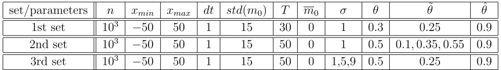
set/parameters n xmin xmax dt std(m0) T m0 σ θ θ˜ θˆ

1st set 103 _{−50 50 1 15 30 0 1 0.3 0.25 0.9}

2nd set 103 _{−50 50 1 15 50 0 1 0.5 0.1,0.35,0.55 0.9}

3rd set 103 _{−50 50 1 15 50 0 1,5,9 0.5 0.25 0.9}

Table 1: Simulation parameters.

LetV(X(t)) = dist(X(t),X), wheredist(X(t),X) denotes the Euclidean distance ofX(t) from the setX. The next result establishes a condition under which the above dynamics converges asymptotically to the set of equilibrium points in a stochastic sense [11].

Corollary 2. (2nd-moment stability) Let a compact set M ⊂ R2 be given. Suppose that for all X 6∈ M

∂XV(X, t)T

−1

c1 +

1

γ2 φ(t)X(t) +h(t)

<−1 2σ

2_∂

xxV(X, t). (25)

Then the dynamics (24) is a stochastic process with 2nd moment bounded.

6. Simulation example

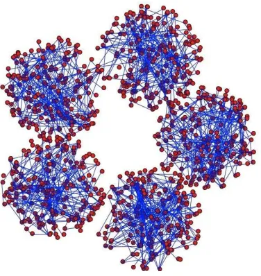
The parameters of the simulation studies are summarized in Table 1. The numerical studies have been conducted considering a thousand of players, five populations, and a discretized set of statesX fromxmin =−50 toxmax = 50. Graph G is a chain, see Fig. 3. The step size is dt = 1 and the horizon is T = 30 in the first set of simulations and T = 50 in the other two sets.

The evolution of the state of each single player is

X(t+ 1) =X(t) + ˆξ(ρk−X) +σ rand[−1,1]. (26)

Note that the above is a discretized version of (24). The initial state x is randomly extracted as explained in the following. Also we consider a discretized version of the second-order consensus dynamics by setting

We assume that the control and disturbance enter in the right-hand-side of a second-order linear differential equation. Using the compact notation

µ•1(t) = m1(t), . . . , m5(t)

T

, µ•2(t) = m˙1(t), . . . ,m˙5(t)

T

,

the dynamics has the form of the second-order consensus dynamics:

µ•1(t)

µ•2(t)

=

I I

−θL −θ˜(L+ ˆθI) +I

µ•1(t−1)

µ•2(t−1)

t= 1,2, . . . , T;

(27) µ•1(0) = (m1(0), . . . , m5(0))T, µ•2(t) = ( ˙m1(t), . . . ,m˙ 5(t))T = (0, . . . ,0)T,

and whereLis the normalized (one for the entries on the main diagonal, and the reciprocal of the degree of node i for each adjacent node of i in the ith row) Laplacian matrix of the communication graph G= (N, E). The elastic and damping coefficients θ, ˆθ and ˜θ are as in Table 1.

We assume m0 to be Gaussian with mean m0 equal to 0. The standard

deviation std(m0) is set to 15. Then, the initial state x in (26) is obtained

from a random realization with density distribution law m0.

Figure 4 shows the time history of the microscopic evolution of each agent’s state. Two phenomena can be observed at two different time-scale. First, on a fast time-scale, agents in each single population k ∈ {1, . . . ,5} synchronize to the local aggregate state ρk. Second, on a slower time-scale, local aggregate states synchronize via second-order consensus dynamics. This explains the inter-cluster oscillations clearly shown in the time plot.

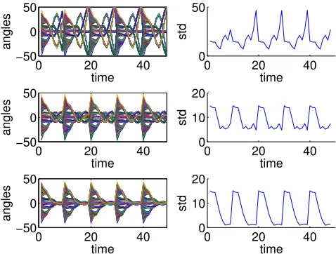
In a second set of simulations we investigate the role of the elastic and damping coefficientsθ, ˆθ and ˜θ. In particular, we simulate three different sce-narios corresponding to an increasing damping coefficient ˜θ = 0.1,0.35,0.55. To investigate how the system responds to periodic impulsive perturbations, we reset the state to the initial value every 10 time units. The resulting time plot is displayed in Fig. 5. On the left column we have the time plot of the microscopic dynamics while on the right column we have the time plot of the standard deviation. The damping effect is visually clear from top to bottom in the plots of the left column.

Figure 3: A thousand of players split into five populations with chain interaction topology.

0 5 10 15 20 25 30

−60 −40 −20 0 20 40 60

power angles

time

Figure 4: Inter-cluster oscillations due to local interactions via second-order consensus.

0 20 40 −50

0 50

time

angles

0 20 40

0 50

std

time

0 20 40

−50 0 50

time

angles

0 20 40

0 10 20

std

time

0 20 40

−50 0 50

time

angles

0 20 40

0 10 20

std

time

Figure 5: Inter-cluster oscillations: the influence of the damping coefficient in the second-order consensus. The plots display the time on the x-axis and the angles (left), and the

standard deviation (right) on they-axis.

7. Conclusions

This paper has studied synchronization via robust mean-field games. We have shown that in less prescriptive environments, where individuals’ behav-iors are not pre-programmed, synchronization may arise as an outcome of strategic thinking, prediction, and local interactions. We have also shown multi-scale phenomena involving fast local synchronization and slow inter-cluster oscillations. Future directions of research involve i) stability analysis under general topologies, ii) the extension of the framework to other coupling effects, and iii) the specialization of the model to electricity pricing.

Appendix

Proof of Theorem 1

To prove (14) let the Hamiltonian and robust Hamiltonian be:

H(x, ∂xvk(x, t), ρk) = inf u

n₁

2

a(ρk−x)2+cu2

+∂xvk(x, t)u

o

= 0,

˜

H(x, ∂xvk(x, t), m) =H(x, ∂xvk(x, t), ρk) + sup w

∂xvk(x, t)w− 1 2γ

2_w2

0 20 40 −50

0 50

time

angles

0 20 40

5 10 15

std

time

0 20 40

−50 0 50

time

angles

0 20 40

5 10 15

std

time

0 20 40

−50 0 50

time

angles

0 20 40

5 10 15

std

time

Figure 6: Inter-cluster oscillations: the influence of the Brownian motion coefficientσ. The

plots display the time on thex-axis and the rotors’ power angles (left), and the standard

deviation (right) on the y-axis.

Differentiating with respect to u and w we obtain (14). To derive (13) note that the second and fourth equations are the boundary conditions and derive from the HJI equation and the evolution of the law of states.

To obtain the first equation, which is a PDE corresponding to the HJI, replace u∗_k appearing in the Hamiltonian (28) by its expression in (14):

H(x, ∂xvk(x, t), ρk) = 1

2a(ρk−x)

2₋ 1

2c

∂xvk(x, t)

2

.

Using the above expression of the Hamiltonian in the HJI equation in (12), we obtain the HJI in (13).

Proof of Theorem 2

Isolating the HJI part of (13) for fixedρk, we have

∂tvk(x, t) +

−₂1_c1 +_2γ12

|∂xvk(x, t)|2 +1

2a(ρk(t)−x) 2₊ 1

2σ 2_∂2

xxvk(x, t) = 0, inR×[0, T[, vk(x, T) = Ψ(ρk(T), x), in R.

(28)

Consider the value function

vk(x, t) = 1 2φ(t)x

2_{+h(t)x+χ(t),}

so that (28) can be rewritten as

1 2φ˙(t)x

2_{+ ˙h(t)x+ ˙χ(t) +−} 1 2c1 +

1 2γ2

[φ(t)2x2 +h(t)2 +2φ(t)h(t)x] +1

2a(ρk(t)

2_+x2_{−2ρk(t)x) +} 1 2σ

2_{φ(t) = 0 in}

R×[0, T[, φ(T) = S, h(T) =−Sρk(T), χ(T) = 1₂Sρk(T)2_.

Since this is an identity inx, it reduces to three equations:

˙

φ(t) +−_c1

1 +

1

γ2

φ(t)2_{+a = 0 in [0, T[, φ(T) = S,}

˙

h(t) +− 1 2c1 +

1 2γ2

2φ(t)h(t)−aρk(t) = 0 in [0, T[, h(T) =−Sρk(T),

˙

χ(t) +− 1 2c1 +

1 2γ2

h(t)2₊1 2aρk(t)

2

+1 2σ

2_{φ(t) = 0 in [0, T[, χ(T) =} 1

2Sρk(T) 2_.

(29)

For the mean-field equilibrium control and worst-case disturbance we have

u∗(x, t) =−1

c1(φ(t)x+h(t)), w

∗_{(x, t) =} 1

γ2(φ(t)x+h(t)). (30)

By averaging the above expressions and substituting in d

dtmk(t) = uk(t) + wk(t) we obtain ˙m(t) = (−_c1₁ + _γ12)(φ(t)mk(t) +h(t)) as in (16). In the

stationary case, i.e. T → ∞, we obtain from (29)

−_c1₁ +_γ12

φ2_{+a= 0,}

−_c1

1 +

1

γ2

φh−aρk= 0,

−1

c1 +

1

γ2

Solving for φ and h yields

h= 1

φ

−_c1

1+ 1

γ2

aρ_k = φ φ2₋1

c₁+

1

γ2

aρ_k =−φρ_k.

Substituting in (30), control and disturbance take the form

u∗(x, t) = 1

c1φ(ρk−x), w

∗_{(x, t) =−} 1

γ2(ρk−x).

Then, mean states of neighbor populations follow the local interaction rule

d

dtmk(t) = uk(t) +wk(t) = φ(

1

c1 −

1

γ2)( P

j∈N(k)mj(t)

|N(k)| −mk(t))

=φ(_c1₁ − _γ12)_|N1_(k)|( P

j∈N(k)(mj(t)−mk(t))).

In other words, local interaction involves a local averaging (the term including the Laplacian defined below) and a local adjustment. For the vector of aggregate states m = (m1, m2, . . . , mp)T, we have the consensus dynamics

˙

m(t) =−Lm(t),where L is the Laplacian matrix defined as

Lkj =

 



φ(_c1₁ − _γ12) j =k,

−φ(1

c1 −

1

γ2)_|N1_(k)| j ∈N(k), j 6=k,

0 otherwise.

Proof of Corollary 1

SinceG= (V, E) is a balanced graph (or undirected graph), we have that the second smallest eigenvalue λ2(φ) is defined by

min 1T_ξ

ξT_Lξ

ξT_ξ =λ2(φ).

The above implies that ξT_{Lξ ≥λ}

2(φ)kξk2.Then

˙

ν(ξ(t)) =−2ξTLξ≤ −2λ2(φ)ξTξ≤ −2λ2(φ)ν(t).

Proof of Corollary 2

LetX(t) be a solution of (24) with initial valueX(0)6∈ X. Sett={inft > 0|X(t)∈ X } ≤ ∞ and let V(X(t)) =dist(X(t),X). For all t∈[0, t]

V(X(t+dt))−V(X(t)) =kX(t) +dX(t)−ΠX(X(t))k − kX(t)−ΠX(X(t))k

= 1

kX(t)+dX(t)−ΠX(X(t))kkX(t) +dX(t)−ΠX(X(t))k

2

From the definition of infinitesimal generator

LV(X(t)) = limdt→0 EV(X(t+dt_dt))−V(X(t))

= limdt→0_dt1 h

E

1

kX(t)+dX(t)−ΠX(X(t))kkX(t) +dX(t)

−ΠX(X(t))k2

− _kX(t)−Π1

X(X(t))kkX(t)−ΠX(X(t))k

2i

≤ 1

kX(t)−ΠX(X(t))k

h

∂XV(X, t)T

−1

c1 +

1

γ2 φ(t)X(t) +h(t)

+ 1 2σ

2_∂

xxV(X, t)

i .

From (25) the above implies that LV(X(t))<0, for all X(t)6∈ M.

Acknowledgments

The author would like to thank the anonymous reviewers for their valuable comments.

References

[1] D. Bauso, H. Tembine, T. Ba¸sar, Robust Mean Field Games, Dynamic Games and Applications, 6(3) (2016) 277–300.

[2] T.K. Dal’Maso Peron, F.A. Rodrigues, Collective behavior in financial markets, EPL (Europhysics Letters), 96(4) (2011).

[3] F. D¨orfler, F. Bullo, Synchronization and Transient Stability in Power Networks and Nonuniform Kuramoto Oscillators, SIAM Journal on Con-trol Optimization, 50(3) (2012) 1616–1642.

[4] D.A. Gomes, J. Sa´ude, Mean Field Games Models - A Brief Survey, Dynamic Games and Applications, 4(2) (2014) 110–154.

[5] High-frequency trading synchronizes prices in financial markets, Said Business Sc., Oxford, http://www.www.sbs.ox.ac.uk/faculty-

research/insights-research/finance/high-frequency-trading-synchronizes-prices-financial-markets (accessed 30.08.16).

[7] M.Y. Huang, P.E. Caines, R.P. Malham´e, Large Population Stochas-tic Dynamic Games: Closed Loop Kean-Vlasov Systems and the Nash Certainty Equivalence Principle, Communications in Information and Systems, 6(3) (2006) 221–252.

[8] M.Y. Huang, P.E. Caines, R.P. Malham´e, Large population cost-coupled LQG problems with non-uniform agents: individual-mass behaviour and decentralized ǫ-Nash equilibria, IEEE Transactions on Automatic Con-trol, 52(9) (2007) 1560–1571.

[9] P. Jia, P.E. Caines, Analysis of Decentralized Quantized Auctions on Cooperative Networks, IEEE Transactions on Automatic Control, 52(2) (2013) 529–534.

[10] J.-M. Lasry, P.-L. Lions, Mean field games, Japanese Journal of Math-ematics, 2 (2007) 229–260.

[11] K. A. Loparo, X. Feng, Stability of stochastic systems, The Control Handbook, CRC Press, (1996) 1105–1126.

[12] R. Olfati-Saber, J.A. Fax, R.M. Murray, Consensus and Cooperation in Networked Multi-Agent Systems, Proc. of IEEE, 95(1) (2007) 215–233.

[13] A. Pluchino, V. Latora, and A. Rapisarda, Compromise and synchro-nization in opinion dynamics, The European Physical Journal B - Con-densed Matter and Complex Systems, 50(1-2) (2006) 169–176.

[14] H. Tembine, Q. Zhu, T. Ba¸sar, Risk-sensitive mean-field games, IEEE Transactions on Automatic Control, 59(4) (2014) 835–850.

[15] H. Yin, P. G. Mehta, S. P. Meyn, U. V. Shanbhag, Synchronization of Coupled Oscillators is a Game, IEEE Transactions on Automatic Control, 57(4) (2012) 920–935.

[16] H. Yin, P. G. Mehta, S. P. Meyn, U. V. Shanbhag, Learning in Mean-Field Games, IEEE Trans. on Automatic Control, 59(3) (2014) 629–644.