L arge S cale D isc r e te -E v e n t
S y ste m s
A n ik a S ch u m an n
THE AUSTRALIAN NATIONAL UNIVERSITY
A thesis submitted for the degree of
Doctor of Philosophy at
The Australian National University
(Vn
ha
I want to thank all people, who have supported this research work in Australia.
My special thanks are due to my supervisors, to Dr Thiebaux for her valuable
guidance throughout my thesis, to Dr Pencole for the many interesting discussions
about existing diagnosis approaches and new ideas and for the enumerative imple
mentation of some diagnosis methods that also allowed me to compare my symbolic
approaches with existing work, and to Dr Huang for pointing me to the interesting
properties of jointrees and his numerous helpful comments on the presented work
with jointrees. My thanks belongs also to Dr Grastien for his valuable feedback on
my entire thesis.
I am also very thankful for the friendly working atmosphere at the Computer
Science Laboratory of the Australian National University and for all new friends,
with whom I share many nice memories.
In this thesis we investigate the diagnosis of large discrete-event systems, where the
task is to determine, on-line, all failures and states that explain a given sequence
of observations. The main challenge here is to deal with the large number of
possible explanations which either results in a very slow diagnosis or, in case they
are compiled off-line, in huge space requirements for the diagnosis algorithms. We
tackle this problem from two angles: On the one hand we present a broad spectrum
of approaches differing in the amount of reasoning and compilation performed off
line and therefore in the way they resolve the tradeoff between the space occupied
by the compiled information and the time taken to produce a diagnosis. This allows
the use of our approach to applications with diverse time and space requirements.
On the other hand we define a framework to assist a human system supervisor in
reducing the number of possible diagnosis explanations by identifying the causes
that make the system so poorly diagnosable and that require a respecification of the
system behaviour. This asks for an extended handling of the
diagnosability
problem
to not only verify whether accurate diagnostic reasoning can be performed on the
system but also to provide all possible reasons of why this might not be the case.
A c k n o w le d g e m e n ts iii
A b s tr a c t v
1 In tr o d u c tio n 1
1.1 Diagnosis - an Informal I n tro d u c tio n ...
1
1.1.1
Why to D iag n o se...
1
1.1.2
What to Diagnose...
2
1.1.3
How to D ia g n o s e ...
3
1.2 Approaches to D iag n o sis...
4
1.2.1
Fault-tree Based M e th o d s ...
4
1.2.2
Expert Systems M ethods...
4
1.2.3
Model-based Methods ...
5
1.3 Frameworks for Diagnosing D E S ...
6
1.3.1
Representation Formalisms for D E S ...
7
1.3.2
Classification of Diagnosis Algorithm s...
8
1.4 Diagnosability of D E S ...
12
1.5 Thesis Motivation & C ontribution...
13
1.5.1
Assisting in the Development of Diagnosable Systems . . . .
13
1.5.2
Diagnosis for Different Requirements of Applications . . . .
15
1.5.3
Increasing the On-line Diagnosis Efficiency...
16
1.6 Thesis O rganisation...
17
2 A S y m b o lic F ram ew ork for D ia g n o sin g D is c r e te -E v e n t S y s te m s 19
2.1
Intro d u ctio n...
19
2.2 Background: Binary Decision D iagram s...
21
2.2.1
Representation of B D D s ...
21
2.2.2
Variable Ordering of BDDs ...
22
2.2.3
Reduction of ordered B D D s ...
24
2.2.4
Application of B D D s ...
25
2.3 Background: Diagnosis Problem and Direct Diagnosis Models . . .
28
2.3.1
Example A pp licatio n ...
28
2.3.2
Modelling of the S y s te m ...
29
2.3.3
Diagnosis Problem for Discrete-Event S y stem s...
32
2.3.4
Spectrum of Direct Diagnosis M o d e ls...
33
2.4 The Symbolic Direct Diagnosis A pproach...
37
2.4.1
Spectrum of Symbolic Direct Diagnosis Models ...
37
2.4.2
Comparison of Symbolic and Enumerative Diagnosers . . . .
53
2.4.3
Symbolic On-Line D iagnosis...
55
2.4.4
S u m m a r y ...
59
2.5 The Symbolic Compiled Diagnosis A p p ro ach ...
60
2.5.1
Spectrum of Compiled Diagnosis M o d e ls ...
60
2.5.2
Experimental Comparison of Model S izes...
71
2.5.3
Correctness of Compiled Diagnosis A pproach...
72
2.5.4
On-line Diagnosis Based on the Compiled Diagnosis Models
77
2.5.5
Experimental Comparison of On-Line Diagnosis Algorithms
79
2.6 Related W o r k ...
80
2.7 Summary ...
83
3 S c a la b le D ia g n o s a b ility C h e c k in g 85
3.1 Introduction...
85
3.2 B ack g ro u n d ...
87
3.2.1
Diagnosability of a Fault in Discrete-Event S y ste m s...
87
3.2.2
Twin Plant Approach for Diagnosability Checking...
88
3.2.3
Jo in trees...
92
3.3.1
Establishing C onsistency...
93
3.3.2
Message Passing ...
95
3.3.3
Propagation of Diagnosability In fo rm a tio n ...
98
3.3.4
An Iterative Jointree A lg o rith m ...104
3.3.5
Jointree Node Selection... 106
3.4 Further Enhancements and M odifications...106
3.4.1
Reduction of Message Sizes ...106
3.4.2
Reduction of Message P ro p ag atio n s... 113
3.4.3
Improvement of Scalability... 115
3.4.4
Diagnosability of a S y stem ... 115
3.5 Relation to Previous W o rk ... 117
3.6 Assisting in the Design of Diagnosable Systems ...122
3.6.1
Computation of Critical P a t h s ...122
3.6.2
Dependencies among Critical P a t h s ...126
3.6.3
Optimal Removal of Nondiagnosability C a u se s... 129
3.6.4
Cost-Driven Computation of Nondiagnosability Causes . . . 130
3.6.5
Extension to Multiple F a u lts...130
3.6.6
S u m m a r y ... 131
4 C o n c lu sio n 133
4.1 Thesis C o n trib u tio n s...133
4.2 Directions for Future W o rk ... 135
In tr o d u c tio n
1.1
D iagn osis - an Inform al In tro d u ctio n
Diagnosis is commonly regarded as the task of explaining an abnormal behaviour of a physical system. This is achieved by monitoring the system and interpreting
its behaviour. It is then the responsibility of the system’s supervisor to use this interpretation in order to choose appropriate actions that remove the system’s abnormalities. This concept is illustrated in Figure 1.1.
Diagnosis
M onitor Interpret
System Supervisor
Figure 1.1: Diagnosis concept
1.1.1
W h y to D ia g n o se
Fault detection and isolation are crucial for a wide range of applications. Several of the significant industrial disasters in the past, such as the major blackout of
New York city, or the Appollo 13 incident could have well been prevented by a timely and accurate detection of a failed relay, or a burnt-out switch [Perrow,
1984]. Thus safety and reliability are two main factors motivating the diagnosis study. Moreover, avoiding undesirable effects of faults, improves the operational
goals of industries, such as increased quality of performance, product integrity, and reduced cost of equipment maintenance and service.
However, given the complex and often non-apparent interactions and coupling
between system components, manual fault detection is extremely difficult if not
impossible. Automated diagnosis mechanisms are therefore needed to monitor large
dynamic applications such as telecommunication networks, business processes, web
services, spatial systems, software components, and power supply networks. This thesis presents several approaches that aim at increasing the efficiency of the on-line
diagnosis to allow for a more timely identification of faults.
1 .1 .2
W h a t to D ia g n o se
In order to perform diagnosis it is necessary to know, how to use the information obtained from the system to reason about the system’s behaviour and its abnor
malities. It is also important to determine which abnormalities are to be diagnosed and passed on to the supervisor. Diagnosis aims to disclose all possible faults. A fault is any abnormality of a system that requires some actions by the system’s
supervisor. For instance, in the context of telecommunication networks a cut cable is considered as fault while a wrongly dialled phone number is not.
Faults can be divided into primary and secondary faults. Primary faults, like
a cut cable, are independent from other faults. Instead, secondary faults occur as consequence of another fault. For example, a blocked telephone might have its
origin in a cut cable.
Moreover, faults are partitioned into permanent and intermittent faults. For
instance, a cut cable is a permanent fault, since it cannot be repaired by the system.
In contrast, a telephone that is blocked due to a cut cable might be repairable. Once the system recognises the problem it might use a reserve cable for the data
transmission. Then the previously blocked telephone is functioning normally again.
One can also distinguish between external and internal faults. External faults
(e.g. a cut cable) are the consequence of some event outside the system, while internal faults (e.g. a blocked telephone) have their origin within the system. Generally the system is able to detect the reason leading to an internal fault, while
it cannot reason about external faults. For example, it is important to detect that a cable is cut, but not how the cable was cut.
The classification of external and internal faults relates to the distinction be tween a system and its environment. The system is composed of all those entities
that are relevant to the diagnostic reasoning. However, a system cannot be viewed
the cable is part of the system’s environment, since the consequences of his actions have to be taken into account. However, he is not part of the system, since his
actual action, that is how he cut the cable, is irrelevant for the diagnostic reasoning.
Finally, different types of fault information can be distinguished: fault detection
which simply states whether the systems is faulty or not, fault localisation where the
faulty components are determined, fault identification where the exact faults that
have occurred are computed, and fault propagation where also the consequences of
faults and their dependencies are considered. Clearly, the richness of the diagnosis result increases from fault detection to fault propagation. In the same way, the
time and space requirements of the diagnosis methods that compute these fault
types increase.
Summarising, diagnosis can be defined as the aim of detecting, localising, iden tifying, or propagating all primary and secondary, permanent and intermittent, external and internal faults of a system, that have any importance to the system’s supervisor. These relevant faults have to be specified beforehand by a human
supervisor.
1 .1 .3
H ow to D ia g n o s e
Firstly, diagnosing faults of a system requires some understanding of the system’s internal structure and its interdependencies. It is necessary to know the conse quences of the faults. If a fault occurs the system usually changes its behaviour,
since it is no longer able to perform all its designed functionality. Secondly, in order to reason about state changes, the system needs to be monitored or observed. This
is done by equipping it with a set of sensors. The kind of sensors required depends on the faults to be diagnosed. For example, a sensor placed at a cable might pro
vide the information, whether the cable is cut or not. By observing this sensor it is
now possible to detect the fault ’cut cable’. In general, the diagnostic task can be described as follows: Given a set or a sequence of observations (sensor readings),
what are the faults that have occurred? This task can be performed on-line or
off-line. In on-line diagnosis, the system is assumed to be in working operation and
the fault information is continuously updated with the events observed. In off-line diagnosis, the system is not in working operation and can be thought of as being
in a testbed. Here the fault information is computed once and for all based on the
A system is said to be diagnosable if the occurrence of every fault can be de tected with certainty after a finite number of subsequent observations. In practice,
industrial systems are not diagnosable due to sensor costs and technological feasi
bility. However, many systems are equipped with some kind of indicators such as alarms or warning lights. By observing these indicators it is possible to determine all faults that might have occurred without knowing whether they have indeed
occurred.
1.2
A p p ro a c h e s to D iag n o sis
Due to its dramatic importance in many application domains, automated diagno sis of large scale systems has received constant and considerable attention from
researchers in the fields of Artificial Intelligence and Control. The existing diag
nosing methods can be classified as fault-tree based systems, expert systems and other knowledge-based, and model-based ones.
1.2.1
F a u lt-tr e e B a se d M e th o d s
A fault tree [Viswanadham & Johnson, 1988] is a graphical representation of the
cause-effect relationship of faults in the system. Based on an observation that
indicates an abnormality of a system, the fault tree is used to reason backwards,
until the root cause of the fault is found. This method is typically applied to alarm analysis in complex system. The main task here is to identify and localise the source of a fault based on simple observations like alarms. However, a fault in one component often causes a faulty behaviour in another component. This leads to a
number of different alarms being emitted which makes it difficult to identify the initial fault. Moreover, the complex problem of constructing the fault tree limits its applicability in practice.
1.2.2
E x p e r t S y s te m s M e th o d s
For systems with subtle and complicated interactions a diagnosis based on expert
systems [Scherer & White, 1987] is often best suited. These systems are tradition
ally rule based. The rules are retrieved from the heuristic knowledge of an expert who relates observations to the faults that produce it. Many of these systems are
based on structures and techniques relating to fault trees [Poucet et al., 1987]. The
required for the diagnosis, the difficulty of validating the systems and their domain dependence.
1 .2 .3
M o d e l-b a se d M e th o d s
It is now widely recognised that building large-scale systems is best achieved by means of model-based representation. That is, rather than relying on procedural
expert knowledge, the system exploits explicit models of individual components, which it combines to automate the reasoning about system wide interactions.
In the classical theory of model-based diagnosis [de Kleer Sz Williams, 1987;
Reiter, 1987], a diagnosis problem consists of a system description, a set of system
components, and observations of the system. The system description specifies the general rules that must be followed in order for the system to function normally.
Here, the system is considered to be static. This means that the observations are
given at a single time point. A diagnosis is defined to be a minimal set A of system
components such that the following two conditions are consistent with the events
observed:
• all components in A are faulty and
• all other components are normal.
Thus it is possible that more than one diagnosis exist where none of the diagnoses
is a subset of another one.
More recently, diagnostic tasks have been successfully developed for some classes
of dynamic systems [Struss, 1997], which allow spontaneous state changes, either triggered by events in the environment, or resulting from the system’s internal dynamics. A good deal of these research efforts has been devoted to model-based
diagnosis of systems modelled as discrete-event systems (DES). DES [Cassandras
h Lafortune, 1999] are dynamic systems with a discrete state space. Its behaviour
is governed by the occurrence of physical events that cause abrupt changes to the state of the system. The majority of large complex systems can be modelled as
DES at some level of abstraction. This discrete-change abstraction is simpler than a continuous-change one and it is still quite powerful, since for diagnostic purposes
many continuous systems can be modelled as discrete using qualitative reasoning
techniques [iwasaki, 1997].
Qualitative reasoning methods enable a program to reason about the behaviour
VI
si
O
52 O
-V I : {open, closed} V 2 : {open, closed} S I : {reached, not reached} S2 : {reached, not reached}
Figure 1.2: Abstract representation of a tank
by conventional analysis techniques. Figure 1.2 illustrates this concept using the
example of a tank. The tank is equipped with two valves V\ and V2 that can be open
or closed and with two sensors Si and S2 that provide the information whether the
water has reached the specified level or not. The tank contains an arbitrary amount
of water and the flow speed of water passing through the open valve V2 varies with
the quantity of water in the tank. Thus this system is continuous. However, for diagnostic purposes it might only be relevant to know, whether the water level is between the two sensors or not, and whether the valves are open or not. In that case the system can be modelled as discrete-event system. The state space consists
of the combination of the valve and sensor settings: V\ x V2 x Si x S2. Now it is no longer possible to retrieve the exact amount of water in the tank, but from a diagnostic point of view this is irrelevant. For instance, given a closed valve V2, a
leak can be diagnosed when the sensor S2 returns reached followed by not reached.
1.3
F ra m ew o rk s for D ia g n o s in g D E S
In the last few years a number of approaches have been developed for the diagnosis
of DES. As stated in the previous section, these approaches are not only applicable to systems that are typically discrete like communication networks or computer
systems, but also to systems that are traditionally continuous. This section first describes the different ways DES can be represented to perform diagnosis tasks. All these diagnosis approaches assume completeness. Then we give an overview of
the research carried out, and we provide several classifications of diagnosis algo
rithms. The main challenge when dealing with large scale systems is the handling of the space/time tradeoff of diagnosis methods. The section therefore closes by
[image:14.519.157.338.133.254.2]1.3 .1
R e p r e s e n ta tio n F o rm a lism s for D E S
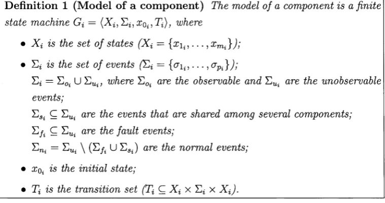
F in ite S ta te M ach in e s
The first framework for diagnosing DES was defined in [Sampath et al., 1995]. Here,
the system can consists of several distinct physical components which might share
certain events. A component can be thought of as the smallest replaceable unit of a
system. The components are modelled as finite state machines (FSMs). The states of the FSM correspond to the component’s internal state and the transitions refer to
its events. Each transition represents the change of states caused by the occurrence
of a single event. Events are divided into sets of observable and unobservable events.
Anything that can be observed by the component using its sensors is modelled as
observable event. All other events are considered unobservable. A subset of the
latter are the fault events. Recalling from section 1.1.2, only those abnormal events
that have any relevance to the system’s supervisor are regarded as faults. Faults are assumed to be permanent. Thus a fault transition indicates only the beginning
of a fault. Note that this approach assumes that it is precisely known how the system behaves if a fault occurs.
Finite state machines can also be used to model DES as set of communicating automata [Roze & Cordier, 2002; Lamperti &: Zanella, 2006]. In this setting, every
component is equipped with input and output terminals to allow interaction among
the components. These connections are described in terms of a structural m.odel,
which is represented as a graph whose nodes are components and whose edges are
the connection links. In addition, a behavioural model, represented as FSM, is used
to describe how each component reacts to incoming messages.
P ro c e s s A lg e b ra
The process algebra approach [Console, Picardi, & Ribaudo, 2002] is very similar to the previous one in that it supports the same compositional method to modelling.
The DES is described with two models: One for the structure of the system, namely the enumeration of the component instances and their connections, and
one for the behaviour of each component type. These models are defined by means
of Performance Evaluation Process Algebra (PEPA) [Hillston, 1996], an algebraic
P e tr i N e ts
DES can also be modelled as Petri nets, which are especially suitable for repre
senting concurrent systems. These nets are described by places, transitions and
directed links between them. Each place may contain several tokens. However, for
diagnostic purposes it is sufficient to consider only places with at most one token
[Aghasaryan et al., 1997]. A marking of a Petri net, that is, an assignment of tokens
to places corresponds to a system state. In order to diagnose a DES, transitions are labelled as observations and certain places are labelled as faults. The system
is faulty if at least one fault place contains a token.
1.3.2
C la ssific a tio n o f D ia g n o sis A lg o r ith m s
Generally, time efficiency is achieved at the expense of space efficiency and vice versa. We now describe how different diagnosis approaches resolve this time/space tradeoff. First we introduce two distinct classifications of diagnosis approaches: simulation-based and diagnoser approaches on the one hand and centralised, de
centralised and distributed approaches on the other hand. Then we present a number of approaches achieving some level of both: time and space efficiency.
S im u la tio n -b a s e d a n d D ia g n o se r b a se d A p p ro a c h e s
Existing model-based methods can be classified into two categories: on-line simu
lation-based approaches compute the diagnosis from the behavioural model of the
system while the latter is working: diagnoser approaches precompute all possible
diagnoses off-line, that is while the system is not working, and retrieve, on-line, the candidate diagnosis explaining the current set of observations. Due to the size of the
supervised applications, existing approaches usually suffer either from poor time performance or from space explosion. Given a system model as a set of individual
components and their interactions, that is, a decentralised model, simulation-based
approaches such as that of Baroni et al. (1999) track the possible system behaviours
on-line as observations become available; the reliance on a decentralised model
makes them space efficient, but the set of possible behaviours is so large that on line computation can be time inefficient. In contrast, diagnoser based approaches
such as that of Sampath et al. (1996) compile, off-line, a centralised system model
into another finite state machine (the diagnoser) which efficiently maps observations
D istrib u ted , D ecen tralised , and C entralised A pproaches
Diagnosis approaches can also be classified into distributed, decentralised and cen
tralised methods1. For the latter, there is one global system model from which
the diagnosis result is computed directly or indirectly [Sampath et al., 1995]. In
decentralised approaches such as [Pencole k Cordier, 2005] there also exists such
a global model, but this is given only indirectly as a set of components. For each
of these components the local diagnosis information is computed and later com bined to obtain the global diagnosis result. Due to the underlying global system model, all events emitted system wide are ordered, which allows the reasoning of
global dependencies among faults. On the other hand, this makes decentralised ap
proaches less suitable for modelling concurrent systems. For the latter, distributed
methods like [Fabre, Benveniste, k Jard, 2002; Wang, Yoo, k Lafortune, 2004;
Su k Wonham, 2005; Qiu k Kumar, 200G] are commonly used. Here only the
observations from the same component or the same subsystem, also referred to as site, are ordered. Mostly, each site has its own local diagnoser associated to
it. The global diagnosis, for instance, is computed by exchanging messages among these diagnosers. This differs from the decentralised approach, in which there is
a centralised coordination of the local diagnosers. In comparison to centralised approaches, decentralised and distributed ones require more diagnosis time while requiring less space. In fact, due to the high space requirements of centralised
methods they can hardly be applied to large scale systems.
D iagn osis A pproaches Tackling th e T im e /S p a c e Tradeoff
Clearly diagnosis methods considering the time/space tradeoff are needed. The
authors in [Roze k Cordier, 2002] approach it by presenting a single framework
using communicating automata which can handle simulation-based and diagnoser
approaches independently. However, most works in this direction aim at combining
these two diagnosis methods. In the following we give a brief overview about them.
In [Debouk, Lafortune, k Teneketzis, 2000] the authors have proposed a frame
work consisting of a set of diagnosers, that each explain the observations from one site. The states of these diagnosers are labelled by sets of global states and fault
labels, and the transitions by the events that can be observed by the site. When
a site observes an event, transitions in the corresponding diagnoser are triggered.
The resulting states are labelled with the diagnosis information of this site. For sites in which the event cannot be observed the local diagnosis information remains
unchanged. The global diagnosis information is computed from the local diagnosis information of all sites using coordinated decentralised protocols.
The work [Garcia et al., 2005] presents another approach that computes the di
agnosis information based on a set of diagnosers. Here the authors target systems
that are composed of subsystems that do not interact with each other and of a com
plex global controller that interacts with several subsystems. The work shows how the global controller, whose events are all observable, can be decomposed to derive a set of minimum local controllers that each only interact with one subsystem.
A diagnoser model is computed for each subsystem and the corresponding local controller. The global diagnosis information can straightforwardly be obtained as the Cartesian product of the corresponding local diagnoser states, since no inter
actions need to be considered. However, this approach is not applicable to systems in which the behaviour of one subsystem has an impact on another subsystem.
The continuous diagnosis approach introduced in [Lamperti & Zanella, 2003a] combines the classical diagnoser approach with the active systems approach. While the latter can only be used off-line, the continuous diagnosis approach enables the on-line computation of diagnosis information made of two parts. The first part is the snapshot diagnostic set, which consists of the faults that are possible after
the last event has occurred. The second part is the historic diagnostic set that contains the complete diagnosis information consistent with the entire sequence of
events observed. When a new event is observed, the new historic diagnostic set is computed based on the former snapshot and historic sets.
In contrast to the previous approaches, Pencole and Cordier (2005) present a decentralised diagnosis framework that computes the complete fault propagation
result and thus also returns all dependencies among faults. The diagnosis algo rithm retrieves a finite state machine containing all events observed and the faults
consistent with them, thereby allowing a deeper reasoning about the occurrence of
faults. The approach is based on a set of subsystems whose states are labelled with a set of graphs each explaining the occurrence of one observation possible in that
state. The subsystem transitions are labelled with the observable events. Once an event is observed, the on-line diagnosis approach proceeds by triggering the corre
synchro-nised to account for the interactions between different components and compute the actual diagnosis information. This approach is very suitable for systems which
require the diagnosis of fault dependencies. Depending on the extent to which state and transition independencies in the diagnosis result can be exploited, an efficient
representation of the latter is also possible [Cordier & Grastien, 2007].
All previous approaches described in this subsection have one thing in common:
they partially compile diagnosis knowledge off-line to allow for a faster on-line di
agnosis. A complete compilation would require the consideration of every sequence
of events and the representation of this compiled knowledge which is infeasible for
large systems. The work of [Lamperti & Zanella, 2006] addresses this problem and
performs an additional compilation on-line based on the actual event sequence ob
served. This special purpose knowledge can then be used to increase the efficiency of similar diagnosis tasks.
For performing diagnosis based on Petri nets, the authors of [Benveniste et
al., 2003] introduce diagnosis nets as a way to encode all solutions of a diagnosis
problem. A solution is a marking of a Petri net, that is, the set of places with a token. In contrast to the diagnoser approach, the computation of the diagnosis nets is performed on-line by relying on Petri net structure only and thus is more space efficient.
Note that the space problem of diagnosis approaches can not only be solved at the expense of computation time, but also at the expense of adding inconsis
tent explanations to the diagnosis result. Such an approach is presented in [Su & Wonham, 2005] where the authors introduce the concepts of global and local con
sistency. Only if the diagnosis result is globally consistent it contains exactly the information that is consistent with the event sequence observed. Otherwise, when
the space efficient local consistency check is performed, it may contain additional diagnosis candidates. Both consistency checks do not consider the computation
time as this approach is entirely off-line.
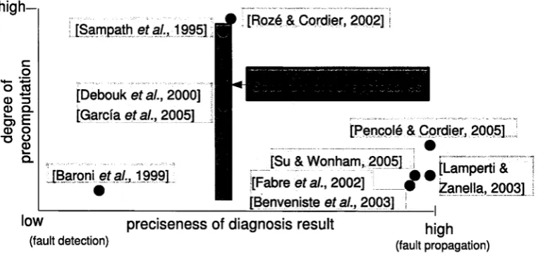
We conclude this section with a comparison of the main approaches presented in this subsection. Figure 1.3 illustrates how these works relate to each other with
respect to the degree of compilation performed off-line and with respect to the
high—
o
*4— 4—*
o co
CD " 5 CD Q_
O) E
CD O T3 <->
CD Q_
[Sampath etal., 1995]
[Debouk et al., 2000]
[Garcia et al., 2005]
[Baroni etal., 1999]
Q
0
O [Roze & Cordier, 2002]
[Pencole & Cordier, 2005] ©
[Su & Wonham, 2005] [Lamperti &
[Fabre et al., 2002]
[Benveniste et al., 2003]
Zanella, 2003]
low
(fault detection)
preciseness of diagnosis result high
(fault propagation)
Figure 1.3: Comparison of diagnosis approaches
1.4
D ia g n osab ility of D E S
A system is diagnosable iff the occurrence of a fault guarantees that it can be detected with certainty after a finite number of subsequent observations. The di
agnosability problem for DES has been introduced in [Sampath et al., 1995] where
the authors solve it by detecting some transition cycles of ambiguous states in a di-
agnoser. The main drawback of this method results from the diagnoser computation which is exponential in the number of states in the global model (determination) and as a consequence is doubly exponential in the number of components in the
system. [Jiang et al., 2001; Yoo & Lafortune, 2002] then propose new algorithms
which are only polynomial in the number of states in G and which introduce the
twin plant method. This method is elegant but impractical for large systems as
the twin plant has a size quartic in the number of system states. Recent work
addresses this issue by building local twin plants for system components, and syn
chronising them with each other until diagnosability is decided [Pencole, 2004]. Still, in the worst case, all local twin plants need to be synchronised, again produc
ing the global twin plant. Moreover all these approaches see the diagnosability
problem as a test on a system and not as a deep analysis of the reasons why a
[image:20.519.62.430.120.305.2]1.5
T h esis M o tiv a tio n & C o n tr ib u tio n
Current model-based diagnosis approaches generally fail when confronted with large
scale discrete-event systems. However, there is an increased need for automatically
diagnosing such systems in many application domains. The work presented in this
thesis aims at reducing the gap between existing and required diagnosis methods
by tackling the efficiency problem at every step, that is
• at design time
by improving diagnosability in order to reduce the number of diagnosis ex
planations that need to be considered on-line
• at compilation time
by taking into account the requirements of the supervised system in order to
choose the best algorithm among a spectrum of approaches and
• at monitoring time
by using symbolic algorithms that speed up the on-line computations and
reduce the space requirements of the diagnosis approaches.
1.5.1
A s s is tin g in th e D e v e lo p m e n t o f D ia g n o s a b le S y s te m s
The gap between existing and required diagnosis methods can be reduced by mak
ing changes to the system itself to reduce the number of diagnosis explanations
consistent with a sequence of observations. This requires in the first place to iden
tify and analyse
all
causes that make the system not diagnosable. Until now the
only work performed in this direction deals with the identification of a single nondi-
agnosable cause. This is done in the context of solving the diagnosability problem.
Now, in order to assist a systems supervisor in respecifying a large scale system we
1. present an
efficient
diagnosability approach which is
2.
scalable
and which
3. computes the
minimum-cost solution
for making the whole system diagnos
able.
constructed we need only synchronise the twin plants in each jointree node, and
all further computation takes the form of message passing along the edges of the
jointree. The properties of the jointree guarantee that after two messages per edge,
the FSMs at all nodes are collectively consistent. To further increase efficiency we
also present additional techniques to reduce the number and size of the messages
computed.
The question of efficiency is also raised in [Cimatti, Pecheur, & Cavada, 2003;
Rintanen & Grastien, 2007; Pencole, 2004]. The first of these works makes use of
symbolic model-checking tools to test a restrictive diagnosability property. Here
the global twin plant is encoded by means of binary decision diagrams. Still, for
large systems even the symbolic representation of the global twin plant might not
be feasible. The second approach can verify the nondiagnosability of a system
using SAT, but cannot verify diagnosability. Finally, the third work shows how di-
agnosability can be decided without computing the global twin plant by iteratively
synchronising local twin plants. This approach forms the basis of our work. How
ever, it is only applicable to systems satisfying a restrictive property. Section 3.5
shows how this approach can be simulated with jointrees and gives a detailed com
parison to our work. Rather than passing messages with bounded event sets the
work presented in [Pencole, 2004] requires the synchronisation of twin plants to
check consistency, which is generally less efficient.
2. When dealing with large scale systems it is essential that our diagnosability
algorithm is scalable in the sense that it is able to provide an approximate solution
to the diagnosability problem whatever the computational resources are.
The
work presented in this thesis is the first one that considers scalability.
3. The number of problems can easily be too high to manually reason about
them. We assist a human system designer by automatically deriving a characteri
sation of ” best” system modifications to restore diagnosability. Here, it is assumed
that cost estimates are available that reflect important characteristics of proposed
system modifications, such as accessibility of subsystems.
gain computational efficiency.
1 .5 .2
D ia g n o sis for D iffe r e n t R e q u ir e m e n ts o f A p p lic a tio n s
We also consider the different needs of applications with respect to their space
and time requirements. Our unified framework therefore consists of a
spectrum
of
approaches which differ in the degree of reasoning performed off-line and by the
nature and the size of the underlying compiled models. In particular, we developed
on-line diagnosis approaches based on the following models (sorted by the amount
of computations performed off-line starting with no compilation):
1. component model,
2. decentralised diagnosis model,
3. global model,
4. centralised diagnosis model,
5. abstracted model,
6. nondeterministic diagnosis model, and
7. diagnoser model.
The model spectrum closest to ours is the one in [Sampath
et al
., 1996]. It
starts with a set of individual component models that are composed to obtain the
global model from which the diagnoser is computed. Here models 1 and 3 are
presented as computation steps. The work describes only one diagnosis approach,
the one based on the diagnoser model.
Models 2 and 4-6 have not been introduced previously and all diagnosis ap
proaches based on them are novel. Figure 1.4 illustrates how our diagnosis ap
proaches relate to existing work. Note, that our methods cannot directly be com
pared to the ones presented in [Debouk, Lafortune, & Teneketzis, 2000; Garcia
et
al.,
2005]. These authors follow a distributed approach and thus use different as
sumptions about the observable events and their order. In contrast our approaches
are centralised (models 3-7) and decentralised (models 1-2).
h ig h
-.o
H— •
O CO CD =3 CD Q .
O) E
CD O
" O o
P
Q .
[Sampath etal., 1995]
[Debouk etal., 2000] [Garcia etal., 2005]
[Baroni etal., 1999]
# [Roze & Cordier, 2002]
O
Spectrum of our approaches
[Pencole & Cordier, 2005]
[Su & Wonham, 2005] [Fabre et al, 2002] [Benveniste et al., 2003]
[Lamperti & Zanella, 2003]
low
(fault detection)
p r e c is e n e s s of d ia g n o sis result high
(fault propagation)
Figure 1.4: Spectrum of our diagnosis approaches contrasted to existing work.
the fault identification information was motivated by the fact that we expected for
such diagnosis approaches the impact of symbolic techniques (see next subsection)
to be the highest.
1 .5 .3
In c r e a sin g th e O n -lin e D ia g n o sis E fficie n c y
To increase efficiency, our diagnosis framework is implemented symbolically us
ing binary decision diagrams (BDDs) [Bryant, 1986]. BDDs enable the compact
encoding and the implicit manipulation of sets of states and transitions. Firstly,
they allow us to reduce the space requirements of models with a high degree of
compilation. Secondly, they help reducing the diagnosis time of approaches with a
low degree of compilation by avoiding the individual consideration of all possible
diagnosis explanations. Therefore, in our approach
• all models are represented as symbolic finite-state machines, and
• all computations are implemented via symbolic operations.
[image:24.519.51.433.81.266.2]spectrum of diagnosis models ranging from component models to diagnoser mod
els. For each of these models, we show how the diagnosis information (i.e. all
faults and system states that explain a sequence of observations) can be derived
on-line, by means of symbolic computations which maximise the benefits of BDDs
for efficiently representing and manipulating large data sets.
1.6
T h e sis O rg a n isa tio n
A S ym bolic F ra m e w o rk for
D iag n o sin g D is c re te -E v e n t
S y stem s
2.1
In trod u ction
For many years, automated fault diagnosis of dynamic event-driven systems has
received constant and considerable attention from researchers in the fields of Artifi cial Intelligence and Control. Given a monitor continuously receiving observations from a system, automated diagnosis aims at identifying faults that explain the ob servations, and at providing an assistance to the operator in charge of the system’s
supervision.
In this chapter, we present a unified symbolic framework allowing for flexible
and efficient diagnosis in applications with different time and space requirements.
In this framework, we define and implement a spectrum of symbolic approaches which resolve the space/time complexity tradeoff in various ways. Our symbolic
techniques are based on binary decision diagrams (BDDs) [Bryant, 1986] which are compact representations of Boolean functions. They enable the encoding and
implicit manipulation of sets of states and transitions, without the need for explicit enumeration.
The chapter consists of two parts. First, to demonstrate the advantages of sym bolic techniques for on-line diagnosis, we show how to directly compute a symbolic representation of well-known models ranging from component models to Sampath
et al. diagnoser 1996, and how to retrieve the diagnosis information based on them.
Furthermore we analyse the time/space tradeoff for the main computation steps
of the symbolic algorithms involved in this “direct" diagnosis approach. Our ex periments on test cases derived from a telecommunication application reveal the
superiority of our symbolic approaches in comparison to the enumerative ones. For instance, we obtain a symbolic diagnoser significantly smaller than the enumerative one, three orders of magnitude faster.
Based on our analysis of the direct approach, we define, in the second part, a symbolic framework that more closely exploits the advantages of BDDs in such
a way that slow operations on models that hardly increase the model’s size are
computed off-line. In contrast to the direct approach, this “compiled” diagnosis approach speeds-up on-line diagnosis by precomputing the diagnosis information
for each component individually. The resulting compiled diagnosis models are all composed of two parts: (i) a decentralised representation of the diagnosis infor mation that is uniform across all models, and (ii) a representation of the system's
behaviour that ranges from a pure decentralised description (comparable to the component models in the direct approach) to a deterministic centralised descrip tion (as e.g. the diagnoser model in the direct approach). Our experiments clearly demonstrate the superiority of the compiled symbolic approach in comparison with the direct one. For instance, the results reveal a significant speed-up of diagnosis time using our decentralised diagnosis model in place of the component-based one.
They also show that one of our compiled models which is considerably smaller than the diagnoser (20 times smaller for our examples), additionally returns a symbolic diagnosis faster than the diagnoser.
This chapter is organised as follows. First we give an introduction to BDDs in Section 2.2. Section 2.3 then defines the diagnosis problem for discrete-event systems and introduces the models on which our direct diagnosis approach is based.
In Section 2.4, we show how these models can be represented by BDDs, describe how we solve the diagnosis problem based on them, demonstrate their performance
2.2
B a c k g ro u n d : B in a ry D ecisio n D ia g ra m s
2 .2 .1
R e p r e s e n ta tio n o f B D D s
Binary decision diagrams (BDDs) [Bryant, 1986] are compact representations of Boolean functions. They enable the encoding and implicit manipulation of sets of
states and transitions, without the need for explicit enumeration. In a range of areas, such as static diagnosis, verification, controller synthesis, or AI planning,
BDD-based representations have given rise to algorithms capable of exploiting the
structure of the system, resulting in significant space and time gains.
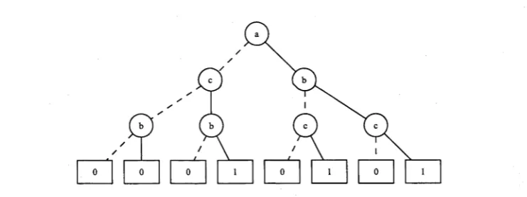
BDDs are derived from Binary Decision Trees (BDTs). A BDT is a rooted,
directed tree with two types of nodes: terminal and variable nodes. The terminal nodes are labelled 0 or 1 and have no outgoing edges. The variable nodes are
marked with a variable v and have two outgoing edges. Figure 2.1 illustrates an
example of a BDT.
Figure 2.1: Binary Decision Tree representing the function / = {aV b)A c.
Dashed lines indicate the low-successor of a node and solid lines refer to the nodes’ high-successor.
Every BDT represents a Boolean function / such that for every terminal node labelled with 0 the function f ( vi , ... ,vn) returns 0 and respectively for every ter
minal node labelled with 1 the function returns 1. The two outgoing edges of a variable node labelled V{ point to the nodes low(vi) and high(vi): low(vi) is the
root of the subtree representing the function / where Vi has been assigned the value
0, while high(v{) refers to the function in which Vi has been assigned the value 1.
The BDT depicted in Figure 2.1 represents the function / = ( aV b)A c.
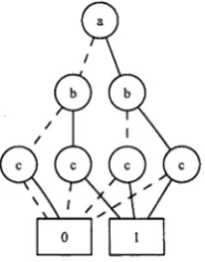
A BDD is a rooted, directed acyclic graph with variable and terminal nodes similar to a BDT. In contrast to the latter, a BDD has only one or two terminal
[image:29.519.106.477.367.506.2]the BDT in Figure 2.1.
o
Figure 2.2: Binary Decision Diagram representing the function / = (aV b)A c.
In order to express operations on Boolean functions in terms of efficient graph algorithms, the BDD needs to be reduced and ordered. This is the case if
1. on all paths of the graph the variables respect a given linear order: V\ < V2 <
. . . < vn
2. no two distinct nodes V\ and v<i have the same variable name and the same
low- and high-successor-. \var{v\) = var{v2)\ A = low A
3. no variable node has identical low- and high-successor.
Henceforth the term OBDD is used to refer to a reduced and ordered BDD. The graph depicted in Figure 2.2 is not an OBDD for three reasons: First, on the path at
the most left the variable ordering is a < c < b while the variables on the right most path are ordered a < b < c. Second, the subtree c with low(c) = 0 and high(c) = 1
is displayed twice by the two right variable nodes c. Third, the two outgoing edges
of the left most variable node b point to the same node. To transform this BDD
into an OBDD. the variables need to be ordered, the duplicated variable nodes removed and the nodes pointing to an identical node need to be deleted. The next two subsections explain the transformation.
2 .2 .2
V a r ia b le O r d e r in g o f B D D s
The shape and size of an OBDD depends significantly on the variable ordering. Figure 2.3 depicts an extreme case of how the ordering affects the size of the graph.
variable ordering ai < b\ < ci2 < 62 < <23 < ^3 (see left graph of Figure 2.3) and once with the ordering <21 < a2 < 03 < 61 < 62 < 63 (see right graph of Figure 2.3).
Figure 2.3: Example of variable ordering dependency
In the first case, the variables are ordered according to their occurrence in the function. From every second level in the graph only two branch destinations are required: one to the terminal node 1 and one to the next level where every
disjunction up to this point yields 0. For the other case it is necessary to construct the complete binary tree for the first three levels, since for each assignment to the
a variables, the function value depends in a unique way on the assignment to the
b variables.
More generally, the OBDD of the function (aq A 61) V . . . V (anA bn) contains 2n + 2 vertices if the variables follow the order a\ < b\ < a2 < 62 < • • • < <2n < bn and 2n+1 vertices if the ordering is aq < 02 < ... < an < b\ < 62 < • • • < bn. Thus choosing an appropriate ordering can dramatically decrease the size of an OBDD.
In [Friedman & Supowit, 1990] the authors present an algorithm for an optimal variable ordering based on a dynamic programming approach. The optimal variable
ordering for the simple BDD depicted in Figure 2.2 is: a < b < c. Figure 2.4 illustrates the ordered BDD1.
However, due to its exponential run time, this algorithm can only be applied
[image:31.519.130.437.166.401.2]Figure 2.4: Ordered BDD representing the function / = (aV b)A c.
to functions with a small number of variables. In fact, as stated in [Bryant, 1986] the problem of computing an ordering that minimises the size of the graph is itself a coNP-Complete problem. In practice the ordering is chosen either manually by
a human with some understanding of the problem domain or automatically by a program using some heuristics.
2 .2 .3
R e d u c tio n o f o rd ered B D D s
The reduction of an ordered BDD requires on the one hand the removal of dupli cated variable nodes and on the other hand the deletion of nodes with identical successors.
A duplicated variable node v\ is deleted following the merging rule. All arcs
leading to V\ are redirected to the identical node. The left graph of Figure 2.5
illustrates the BDD for the function / = [aV b) A c after all identical nodes have been removed.
A node v2 for which both outgoing edges lead to the same node can be deleted by
applying the deletion rule. All incoming edges to v<i are redirected to the common
successor node. Figure 2.5 presents the OBDD of the function f = (a V b)A c.
The two reduction rules are sufficient to obtain the canonical representation
for each function and each variable ordering [Bryant, 1986]. Applying these rules levelwise bottom-up, leads to an efficient reduction of BDDs. The authors in [Siel-
[image:32.519.203.296.132.251.2]ing Sz Wegener, 1993] present a reduction algorithm with linear run time 0 (|G |),
where |G| denotes the number of nodes in the BDD G. Note that it is possible if
not necessary to reduce a graph during its construction. Thus the computation of large unreduced BDDs can be avoided.
Figure 2.5: Ordered BDD without duplicated variable nodes representing the func
tion / = (a V b) Ac (left) and reduced and ordered BDD representing the function
/ = (a V b) A c (right).
a Boolean function. Since identical subexpressions in an OBDD are represented
only once, an OBDD can be exponentially more compact than its corresponding
truth table representation. For instance, the OBDD for the constants 0 and
1 respectively consists of exactly one terminal node. The uniqueness property implies the possibility of testing in constant time whether an OBDD represents a tautological function in which case the OBDD consists of the single terminal node 1
or whether the represented function is satisfiable in which case the OBDD consists of any structure other than a single terminal node 0. In contrast, these problems are NP-complete for Boolean expressions. In the remainder of this chapter we will
use BDDs to denote ordered BDDs.
2 .2 .4
A p p lic a tio n o f B D D s
BDDs are useful in compactly representing finite state machines (FSMs). To en
code state and event sets it is necessary to introduce Nr(Q) = [log2 |Q|"| Boolean
variables for each set Q. Thus the events labelling the transitions can be encoded
with the Boolean variables 6E = { b f, . . . , 6Er(^ } and the states with the variables
bx = {bx , . . . , &)vr(x)}- A state of the FSM is then simply given by a Boolean function (represented by a BDD) over these state variables. For instance, in a 6 state FSM, the state x 2 would be given by the conjunction ~>bx A bx A -*bx , and
the set of states {x2, x5} by the DNF (~>bx A bx A ~>bx ) V (bx A ->bx A bx ).
Transitions require the introduction of another set of state variables bx> =
{bx ' ,. . . , bx 'r^y) }, called the primed variables, which are used to represent the tar
BOOL IsD efibdd)
• Returns true if bdddoes not represent false
BD D GetConj (bdd)
• Returns a single arbitrary disjunct (a conjunction of literals) of the DNF represented by bdd. for example:
bdd (bi A 62) V (-'fri A -162)
GetConj(bdd) = (61 A 62)
BD D AbstractVar(bdd, { 6 1 ,..., 6m})
• Deletes all occurrences of the Boolean variables {6l5. . . , 6 m} from bdd, for example:
bdd «— (61 A 62 A 63) V ( ~'&i A —162 A ->63)
AbstractVar(bdd, {63}) = (61 A 62) V (— A -i62)
BD D ExtractVar(bdd, { 6 1 , , 6m})
• Deletes all occurrences of the Boolean variables th a t are NOT { 6 1 ,..., bm} from bdd, for example:
bdd <— (b\A 62 A 63) V ( ~>6i A ~d>2A ■“>63)
ExtractVar(bdd, {61,62}) = (61 A 62) V (—161 A -i62) BD D SwapVar(bdd, {a1?. . . , an}, {6l5. . . , 6m})
• Swaps the Boolean variables (ai, 61), . . . , (an,6m) in 6dd, for example:
bdd *— (61 A -162 A 63) V ( —'61 A 62 A —163)
SwapVar(bdd, {61}, {62}) = (62 A —>61 A 63) V (-162 A 61 A ->63)
[image:34.519.55.428.129.657.2]in a FSM consisting of 6 states and 3 events, the transition t = x2 —L £5 can be encoded as t = (->63 A bx A -<6*) A (->62 A b f) A (fof' A ->bx A 6* ). The transition
relation, i.e, a set of transitions T, can be given as a DNF which the BDD data structure will hopefully greatly reduce.
When using the compact representation and efficient manipulation of BDDs in the context of our direct diagnosis methods, our representation of the com
ponent models will essentially follow the usual symbolic FSM representation de
scribed above, while all other models will be derived from these component models via symbolic computations. This will be detailed in the next section. To in
crease the readability of our symbolic algorithms, we introduce some basic BDD
operations shown in Table 2.1. Note that the table contains two similar func
tions: AbstractVar and ExtractVar. Let bdd denote a BDD defined over the
set of variables B, and let V be a subset of B. The following equivalence holds:
AbstractVar (bdd , V ) = ExtractVar (bdd, B \ V).
Algorithm 1 illustrates the use of most of these BDD operations to compute all
states X reach that are reachable from a state set X via the transitions in T. Note that we give identical names to sets and to the corresponding Boolean functions,
e.g. X . This should not cause confusion.
As described above, X is defined over the Boolean variables bx and T is defined
over the variables 6s U bx U bx '. The reachable state set is computed using breadth
first search. Initially X reach is set to false and the set of states X new from which transitions still need to be triggered is set to the start states X (lines 2-3).
Algorithm 1 C o m p R e a c h ^ ,b x ,bx , X , T )
1: INPUT: state set X , transition set T and the Boolean variables over which they are defined
Initialise
2. X reach * false
3- X new * X
4: while there are new states (that is as long as I s D e f ( X new)) do
5: T -1 newi— X new A T
6: X t a r g * ExtractVar(Tnew, bx>) 7: X t a r g i SwapVar (Xtarg, bx , bx ')
8: X n e w i X t a r g A ““1X r each
9: X r e a c h — X r e a c h V X new
10: end while
Until a fixed point is reached, all transitions Tnew starting in X new are triggered
(operator A) (line 5) and the targets states that have not yet been encountered
are added to X reach (operator V)(line 9). To obtain the target states X targ of
the transitions Tnew, we abstract the latter from its start states and events using
function ExtractVar (line 6). Originally the targets X targ are defined over the
variables bx>. In order to compute the transitions starting in states of X targ in
the next loop iteration, we swap the state variables to represent X targ over the
variables bx (line 7). Finally, to guarantee the termination of the algorithm, we
only consider those targets from which transitions have not yet been triggered.
Hence we subtract all previously encountered states X reach from X targ (operator
A-i)(line 8).
Note that all transitions starting from a set of states can be computed at once
(line 5). In fact, the whole procedure does not require the consideration of individ ual states or transitions. It is this property of BDDs that we aim to exploit in the context of on-line diagnosis.
2.3
B a c k g r o u n d : D ia g n o s is P r o b le m a n d D ir e c t
D ia g n o s is M o d e ls
This section describes how we model the systems to be diagnosed. Then we define the diagnosis problem and a spectrum of models, the direct diagnosis models, that can all be used to solve this problem. To illustrate our concepts we start by introducing an example application which we will use throughout this chapter.
2 .3 .1
E x a m p le A p p lic a tio n
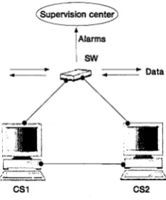
Our example is derived from a telecommunication network [Roze & Cordier, 2002],
A supervision centre is in charge of continuously monitoring the system; it receives a
flow of alarms and analyses them on-line to identify possible faults (see Figure 2.6). The supervised system is composed of two control stations (CS1 and CS2) and one
switch (SW). The switch is used to route data through the network. The purpose of the control stations is to manage the switch by reconfiguring it or reinitialising
it. Only one control station manages the switch at a given time, the other is for replacement in case the station in charge fails to work.
A fault SWfail can occur in the switch. In that case both control stations