A Bayesian decision-theoretic model of sequential experimentation with delayed response

White Rose Research Online URL for this paper: http://eprints.whiterose.ac.uk/110768/

Version: Accepted Version

Article:

Chick, Stephen, Forster, Martin orcid.org/0000-0001-8598-9062 and Pertile, Paolo (2017) A Bayesian decision-theoretic model of sequential experimentation with delayed response. JOURNAL OF THE ROYAL STATISTICAL SOCIETY SERIES B-STATISTICAL

METHODOLOGY. pp. 1439-1462. ISSN 1369-7412 https://doi.org/10.1111/rssb.12225

[email protected] Reuse

Items deposited in White Rose Research Online are protected by copyright, with all rights reserved unless indicated otherwise. They may be downloaded and/or printed for private study, or other acts as permitted by national copyright laws. The publisher or other rights holders may allow further reproduction and re-use of the full text version. This is indicated by the licence information on the White Rose Research Online record for the item.

Takedown

If you consider content in White Rose Research Online to be in breach of UK law, please notify us by

Experimentation with Delayed Response

Stephen Chick

, Martin Forster,

Paolo Pertile

November 30, 2016

Abstract

We propose a Bayesian decision-theoretic model of a fully sequential experiment in which the real-valued primary end point is observed with delay. The goal is to identify the sequential experiment which maximises the expected benefits of technology adoption decisions, minus sampling costs. The solution yields a unified policy defining the optimal ‘do not experiment’/‘fixed sample size experiment’/‘sequential experiment’ regions and op-timal stopping boundaries for sequential sampling, as a function of the prior mean benefit and the size of the delay. We apply the model to the field of medical statistics, using data from published clinical trials.

Keywords: Bayesian inference; Clinical trials; Delayed observations; Health economics; Sequential experimentation

∗_{Corresponding author. Novartis Chair for Healthcare Management, Technology and Operations} Man-agement Area, INSEAD, Boulevard de Constance, 77300 Fontainebleau, FRANCE. (33) 1.60.72.41.57. [email protected]

1

Introduction

The ethical and economic advantages of sequential and adaptive clinical trial designs are well documented (Armitage, 1975; Berry, 1985; Whitehead, 1997; Jennison and Turnbull, 1999). It is also common to observe data on patient outcomes some time after treatment has taken place. For example, Brown et al. (2000) measured outcomes immediately following surgery and again at one and twenty four hours post-surgery; Connor et al. (2015) measured the primary end point at 90 days and Moses et al. (2003) measured outcomes over one year. Less well researched is the question of how sequential experiments should be adjusted when the primary end point arrives with delay.

This question is especially important given the increasing policy interest in sequential and adaptive trial designs (European Medicines Agency, 2006; US FDA, 2010). Concern about avoiding unnecessary recruitment to the trial, past the point at which evidence is deemed to be conclusive, means there is a growing focus on valuing the cost of carrying out research, to-gether with the benefits that accrue to trial participants and patients who may benefit from a new technology (Lewis et al., 2007; Willan and Kowgier, 2008; Pertile et al., 2014). Indeed, the UK National Institute for Health and Care Excellence (NICE, 2012) examines cost and effectiveness when making tradeoffs in care, and the value-based health movement (Porter, 2010) calls for increased attention to the health benefits obtained for a given level of expenditure.

Hampson and Jennison (2013) provide an overview of the emerging literature on group se-quential trial design with delay. They derive new, frequentist, delayed response group sese-quential tests for two-treatment comparisons of mean efficacy which minimise the trial’s expected sam-ple size, subject to meeting prespecified type I and type II error probabilities. The authors derive their optimal stopping rules by solving Bayes decision problems using dynamic programming. Broglio et al. (2014) present a Bayes adaptive design which stops recruitment to a trial if the pre-dictive probability of success upon immediate cessation of recruitment and follow-up of pipeline patients exceeds a predefined probability, or if the predictive probability of success at the maxi-mum sample size is lower than a predefined futility probability.

In discussing Hampson and Jennison (2013), Draper (2013) suggests that solving a Bayesian decision-theoretic model, whose utility function measures outcomes on a clinically relevant scale (such as the Quality Adjusted Life Year, or QALY, e.g. see NICE 2012) could provide real gains over the type I/type II error probability scale. Burman (2013) also advocates use of a Bayesian decision-theoretic framework which measures explicitly the cost of sampling and the value of trial results and which incorporates a prior distribution for the expected outcome.

well as expected benefits which accrue to the patients who benefit from the adoption decision. Discounting of future costs and benefits is permitted, so that the model may be applied to health technology assessments such as those considered by NICE. To the best of our knowledge, ours is the first to combine all of these features within a unified framework.

Section 2 presents and solves the model for the case of a known sampling variance. Section 3 highlights the main features of the optimal policy using an illustrative example. Section 4 con-siders the case of an unknown sampling variance. Section 5 presents an application using data from a published clinical trial for drug-eluting stents and assesses the operating characteristics of the model’s optimal policy. Directions for future research are presented in section 6. Appendix A and the Online Supplementary Material (OSM, Appendix S) provide mathematical proofs and further details on our methods, as well as an additional application. Matlab code which

imple-ments these computations is provided athttps://github.com/sechick/htadelay.

2

The model

We consider a two-armed, sequential clinical trial in which study units are allocated at random, and in a pairwise manner, to either a control (the current best available standard) health technol-ogy or a new one. There is a sampling costc∈R_{≥0 ≡[0,∞)per pairwise allocation made. The}

purpose of the trial is to evaluate which technology should be used to treatP _∈ R_{>0 ≡ (0,∞)}

patients upon stopping the trial. A one-time switching costI _∈R_{≥0is incurred if the decision is}

made to adopt the new technology. No such cost is incurred if the decision is made to continue with the standard technology.

Effectiveness is denoted by the random variable EN ∈ Rif a patient is assigned to the new technology andES ∈ Rif the patient is assigned to the standard one. The patient-level costs of using each technology are the random variablesCN ∈R≥0 andCS ∈R≥0. It is assumed that all patients complete their assigned course of treatment, there is no loss to follow up, and EN, ES,

CNandCSare observed without measurement error.

Following standard approaches in Bayesian decision-theoretic models (see, for example, Berry and Ho 1988, Lewis et al. 2007 and Pertile et al. 2014) and in line with the suggestion of Burman (2013), a common unit of measurement is used to value benefits and costs. We as-sume that effectiveness is valued in monetary terms, using survey data or information provided by a regulatory body such as NICE (for example, NICE values one Quality Adjusted Life Year (QALY) at between £20,000 and £30,000). Define λ ∈ R_{>0 as the monetary value of one unit}

of effectiveness. Then the individual level incremental net monetary benefit ( INMB ) of the new technology versus the existing one for pairwise allocationiis:

Xi =λ(EN,i−ES,i)−δCE(CN,i−CS,i), (1)

whereδCE = 1if the experiment assesses cost-effectiveness andδCE = 0if it assesses effectiveness only. It is assumed thatXi _{∼ N}(W, σ2

X),i=1,2, . . . , Tmax, whereTmax ∈Z>0 is the maximum

number of pairwise allocations which can be made in the trial. W is assumed to be unknown andσ2

related data. For example, choice of the so-called ‘effective sample size’ of the prior distribution, n0 =σX2/σ02, might be guided by the sample size of a related Phase II clinical trial or pilot study. O’Hagan et al. (2006) provide additional guidance on specifying prior probability distributions.

The annual rate of accrual to the trial is assumed to be constant and equal toR ∈ R_{>0. In}

contrast to the model of Pertile et al. (2014), the Xi arrive with a delay of τ ∈ Z≥0, τ < Tmax, pairwise allocations, at which point they are used to update the prior/posterior distribution forW in a sequential manner. The number of pairwise allocationsτ of delay therefore depends on the rate of accrual, R, and the time delay in observing the outcome. Future benefits and costs may be down-weighted using a discount rate, defined at the level of one pairwise allocation asρ˜_≥0.

2.1 The decision problem in discrete time

DefineT _{≡ {0,1, . . . , Tmax}, and defineT ∈} T_{as the time at which pairwise allocations cease}

to be made. DefineT¯ _{≡ {0,1, . . . , Tmax+τ}as the set of equally spaced times where pairwise}

allocations and/or a choice to adopt one of the two technologies may be made.

At eacht _∈ T_{\{Tmax}, an actionatis chosen from the set of available actions,A ≡ {0,1},}

such that at = 1 denotes choosing to make a pairwise allocation (so that T > t) and at = 0 denotes choosing not to make a pairwise allocation. It is assumed that, once pairwise allocations cease to be made, sampling cannot be restarted: at the first occurrence of at = 0, pairwise allocations cease (so thatT =tandat= 0for allt > T).

Fort _≤τ,at is chosen only on the basis of prior information. Forτ < t < Tmax, the action can be a function of the _{Xi_}1≤i≤t−τ. For t = τ, . . . , Tmax − 1, the ordering of events is as follows: actionat is chosen; realisationXt+1−τ = xt+1−τ is observed; prior distribution forW is updated. If sampling continues as far ast =Tmax,T =Tmaxand sampling stops.

Once sampling is stopped, one must wait to observe all outcomes for the ‘pipeline subjects’ – those who have been treated but whose outcomes have yet to be observed – before making the technology adoption decision. Define_{D ∈ {}N,S_}as the decision concerning whether to choose the new technology (N) or the standard (S). This adoption decision is made at time0ifa0 = 0, because no pairwise allocations will be made. It is made at timeT+τ,T >0, ifa0 = 1, because of the delay.

More compactly, the adoption decision is made at time1T >0(T+τ), where1F is the indicator function, equal to 1 if the eventF is realized and 0 otherwise. The expected reward from selecting technology _D, ignoring the cost of sampling and discounting, is 1D=N(P W −I). A policy π

is a dynamic method of deciding, at each time t, to take an action from _A using the history of choices and realisations that have so far accrued, and a technology adoption decision from _D. The objective is to establish a policyπ∗ which maximises the expected reward of the sequential sampling process and adoption decision.

nt=n0+ (t−τ)+, andYt =µ0n0+ (t−τ)+

X

i=1

Xi, (2)

where(m)+ _{= max(0, m)and the sum is equal to 0 if the upper bound for the summation is 0.} The posterior distribution forW at timethas a normal distribution

W| Ft∼ N(µt, σX2/nt), where: (3a)

µt=Yt/nt. (3b)

We may use(yt, nt)as a sufficient statistic forW conditional onFtand we use(yt, t)as a state because it also provides information about the number of pipeline subjects.

A policyπdefines a mappingf(yt, t) :R_×T_{\{Tmax} → Afrom states to deciding whether}

to make a pairwise allocation, which in turn determinesT. A policyπalso specifies the choice of the new technology or standard,_{D ∈ {}N,S_}, as discussed above.

By construction, T is a stopping time with respect to the filtration_F taking values inT_{; D}

is_F1T >0(T+τ)-measurable andπis measurable with respect toF. LetΠbe the set of all policies

which are so measurable with respect to_F. We writeE_{π to denote the expectation with respect}

to the measure induced byπon the sequence of observations and decisions, andE_{to indicate the}

expectation when it does not depend onπ. Table 1 summarizes the principal notation.

The expected reward from a policy π _∈ Πdepends on the parameters of the prior distribu-tion (µ0, n0), and is determined by the cost of sampling, benefits to patients during the trial (if permitted), and benefits from the technology adoption decision:

Vπ(µ0, n0) =Eπ

"(_T−1 X

t=0

−c+δonXt+1 (1 + ˜ρ)t

)

+ 1D=N(P W −I) (1 + ˜ρ)1T >0(T+τ)

µ0, n0

#

. (4)

Here, δon = 1 if the benefits to patients participating in the trial (in addition to the P post-trial patients) are to be included in the reward function (known as ‘online learning’). δon = 0 if rewards for participants are not to be included in the reward function (‘offline learning’). Traditional trials set δon = 0 implicitly. The term 1T >0(T + τ) indicates that a penalty for discounting is only relevant for the terminal reward if at least one pairwise allocation is made.

The objective is defined to be that of finding a policyπ∗ _{∈Πsuch that}

Vπ∗

(µ0, n0) = sup

π∈Π

Vπ(µ0, n0). (5)

It will be useful to analyze three distinct stages of the trial in order to characterise the op-timal policy. These are illustrated in Figure 1. During stage I (t ∈ {0,1, . . . , τ −1}) pairwise allocations are made sequentially and no outcomes are observed, owing to the delay. During stage II (t _{∈ {}τ, τ + 1, . . . , T ₋ 1_}) pairwise allocations are made, realisations xt+1−τ for pipeline subjects arrive sequentially and are used to carry out Bayesian updating. Duringstage III

(t_{∈ {}T, T + 1, . . . , T+τ_}) no pairwise allocations are made, observations on pipeline subjects

P _∈R_{>0 Number of patients to receive technology once adoption decision made}

I_∈R_{≥0 Fixed cost of switching to the new technology from standard technology}

X _∈R(random variable) Incremental effectiveness/net monetary benefit of new over standard

σ2

X∈R>0 Variance ofX

W _∈R Expected value ofX

µ0∈R, σ02∈R>0 Mean and variance of prior distribution forW n0=σX2/σ20 Effective sample size of prior distribution

τ∈Z_≥0,τ < Tmax Delay in observing realisation of pairwise allocation (in pairwise allocations)

Tmax∈Z>0 Maximum number of pairwise allocations which can be made

T_{≡ {0,1, . . . , Tmax}} Set of potential patient pairs to be allocated

T_{I≡ {0,1, . . . , τ−1}} Recruitment of trial participants only

T_{II≡ {τ, . . . , Tmax−1} Parallel recruitment and Bayes updating possible}

¯

T_{≡ {0,1, . . . , Tmax+τ} Set of times when pairwise allocations and/or treatment choice may be made}

at∈ A ≡ {1,0} Action to make a pairwise allocation (at= 1) or not (at= 0),t∈TI∪TII T _∈T _{Time at which pairwise allocations cease to be made (stopping time)}

D ∈ {N,S_} Decision to adopt new or standard, having observed all realisations

π Sequence of sampling decisions and an adoption decision

Π Set of policies whereT _≤Tmax

F= (_Ft)t∈T¯ Natural filtration defined by the observations seen through timet

E_π;E Expectations: with respect to filtration induced byπ; independent ofπ nt=n0+ (t−τ)+ Effective sample size of posterior distribution astth pairwise allocation is made

Yt=µ0n0+P(t−τ)

+

i=1 Xi Cumulative sum for posterior mean

µt=Yt/nt Posterior mean ofW whentpairwise allocations have been made

Zt,u Posterior mean to be obtained, givenFtandu‘pipeline’ observations to arrive

c_∈R_>0 Recruitment cost of making one more pairwise allocation

R_∈R_>0 Annual rate of recruitment to the trial ˜

ρ_≥0 Discrete time discount rate at level of one pairwise allocation

λ Monetary value of one unit of effectiveness (e.g., £30,000 / QALY)

δon 1 = ‘online learning’; 0 = ‘offline learning’

Table 1: Table of principal notation.

In sections 2.1.1–2.1.3 we formulate a dynamic program (Bertsekas and Shreve, 1978) by developing Bellman’s equation for the expected reward in reverse time from stage III to stage I. Section 2.2 justifies how an optimal policyπ∗ _{∈ Πcan be determined from Bellman’s equation} and provides further results for two special cases. Section 2.3 introduces the method that we use to solve the problem.

2.1.1 Optimal rewards in stage III

Stage III is entered when recruitment to the trial stops at timeT. The optimal expected reward upon entering stage III depends on theu= min(T, τ)pairwise allocations in the pipeline: u=T if stopping takes place during stage I, andu =τ if it takes place during stage II. LetZt,u be the posterior expected INMB at the patient level, given the information to timetand thatuoutcomes are still to be observed. Then in our setting:

Zt,u _≡E_{[W| Ft, Xt−u+1, Xt−u+2, . . . , Xt]∼ N}

µt,σ

2 X nt

u (nt+u)

0 t T

Stage I

(recruitment only)

Stage II

(recruitment and updating)

Stage III

(updating only)

T+t

Figure 1:Stages of the problem with stopping timeT and delayτ.

An adoption decision can be made immediately if T = 0 because no trial takes place. If

T > 0, the last of the observations on pipeline subjects will be observed τ time units after

stopping. Once all outcomes on pipeline subjects are observed, it will be optimal to adopt the new technology (_D=N) ifP ZT,min(T,τ)−I >0and the standard one (D=S) otherwise. Define G:R_×N_{0 →}R_{as the optimal discounted expected reward following a decision to stop at time}

T =tand wait for the observations on pipeline subjects before making an adoption decision:

G(yt, t) = (1 + ˜ρ)−1t>0τ_E

[ (P ZT,min(T,τ)−I)+|YT =yt, T =t]. (7)

2.1.2 Bellman’s equation for stage II

For stage II, let T_{II ≡ {τ, . . . , Tmax−1}be the set of times at which pairwise allocations can}

be made, outcomes are being observed and Bayes updating is taking place. The decision about whether to make the next pairwise allocation is based on a comparison ofGin Eq. (7) with the expected reward of making that allocation, observing the outcome of the next pairwise allocation in the pipeline, and continuing to behave optimally on the basis of that outcome. DefineB(yt, t) :

R_×(T_{II ∪ {Tmax}) →} R _{as having the maximum value of the expected reward for the next}

allocation decision, given that t pairwise allocations have been made and (t −τ) have been observed, resulting in a posterior mean ofyt/nt. Then Bellman’s equation in stage II is:

B(yt, t) = maxnG(yt, t), −c+δon(yt/nt) (8a)

+ (1 + ˜ρ)−1E_{π[B(yt+Xt+1−τ, t+ 1) | yt, t]}o_{, t∈}T_II,

B(yTmax, Tmax) =G(yTmax, Tmax). (8b)

If the second term in the maximand of Eq. (8a) exceeds the first, at = 1 and stage II continues with an additional pairwise allocation so thatT > t. For the first occurrence at which the first term exceeds the second, at =0 and the stopping time is T = t. If the first term never exceeds the second, the trial runs to the maximum sample size (T =Tmax).

2.1.3 Bellman’s equation for stage I

nt =n0fort∈TI≡ {0,1, . . . , τ −1}. Thus,

B(yt, t) = max

G(yt, t),−c+δon(y0/n0) + (1 + ˜ρ)−1B(y0, t+ 1) , t∈TI. (9)

The special case ofτ = 0is modeled by lettingT_{Ibe the empty set, letting stage II commence}

at timet= 0, and noting the simplificationG(yt, t) = (P yt/nt−I)+_{in Eq. (7).}

2.2 Characterization of the optimal policy

This section shows that a policyπ ∈Πis optimal for the sequential sampling problem in Eq. (5) if it selects (almost surely) the argmax of Bellman’s equation in Eqs. (8) and (9). It provides additional structural results which characterise the optimal solution for some special cases.

We first observe that, for the special case of free, undiscounted sampling (c= 0,ρ˜= 0) with offline learning (δon = 0), the following policy is optimal: sample as much as possible (T = Tmax) and select the new technology if the posterior mean net reward is positive (P µT+τ−I >0) once all outcomes have been observed, and the standard otherwise. This result is trivial from the observation that information, in expectation, has a nonnegative value.

The special case of offline learning (δon = 0), positive discounting (ρ >˜ 0), no sampling costs (c = 0) and no time delay (τ = 0) reduces to the special case of Chick and Gans (2009) for comparing a known alternative (standard) with known mean reward0with an unknown al-ternative (new technology) with unknown mean reward P W ₋ I. The special case of offline learning (δon = 0), positive sampling costs (c > 0), no discounting (ρ˜= 0) and no time delay (τ = 0) reduces to the special case of Chick and Frazier (2012) for the same comparison. We now draw upon, and extend, those results to account for general costs (that is, at least one ofcand

˜

ρpositive), delayed responses (τ ≥0), as well as both offline and online learning (δon ∈ {0,1}). It will be useful to define V¯ as the expected reward of an oracle who adopts the prior dis-tribution for W and who will become aware of the true value of W immediately before start-ing the trial. The oracle then has the option to adopt one of the two technologies immedi-ately, based on that information, and still run patients through the trial if there exists online learning and the expected reward for those patients exceeds the cost of sampling them. Let Tmax,ρ˜ = PtT=0max−1(1 + ˜ρ)−tbe the discounted maximum number of pairwise allocations in the trial. Then, givenµ0 andn0 and prior to knowingW, define:

¯

V(µ0, n0) = E[(P W −I)++δon(W −c)+Tmax,ρ˜|µ0, n0]. (10)

The termE_{[(P W −I)}+_{|µ0, n0]is the oracle’s expected reward from selecting the best}

tech-nology immediately before executing the trial (that is, assuming no penalties for discounting). The termE_{[δon(W −c)}+_{Tmax,ρ˜|µ0, n0]is the oracle’s expected reward from sampling all patient}

pairs if online learning is permitted and such sampling has positive net reward.

Proposition 2.1 For policiesπ∈Π:

Vπ(µ0, n0) = ¯V(µ0, n0)−V˜π(µ0, n0), (11)

whereV˜π_(µ

0, n0)≡Eπ[Kπ+Sπ+Lπ|µ0, n0]and the following terms are each non-negative:

Kπ ≡

T−1

X

t=0

Kπ,t, whereKπ,t= (c−δon(W −(W −c)+))/(1 + ˜ρ)t, (12a)

Sπ ≡

Tmax−1

X

t=T

δon(W −c)+/(1 + ˜ρ)t, (12b)

andLπ ≡(P W −I)+−1D=N(P W −I)/(1 + ˜ρ)1T >0(T+τ). (12c)

By Eq. (11), a policy π maximisesVπ _{if and only if it minimisesV˜}π_{. Minimisation ofV˜}π is itself a sequential optimal stopping problem, in which_Kπ is an opportunity cost of sampling,

Sπ is a residual penalty in the presence of online learning if the stopping time is not equal to the oracle’s stopping time and Lπ is the opportunity cost of selecting a potentially suboptimal technology_Dafter all outcomes are observed, accounting for any discounting owing to the delay. This observation, together with the nonnegativity of_Kπ,Sπ, andLπ, allows us to use Bertsekas (2005) and Bertsekas and Shreve (1978) to characterise the optimal policy with Bellman’s equa-tion.

Proposition 2.2 If all decisions of a policyπ∈Πattain the maximum in Bellman’s equation in Eq. (9) for stage I decisions and in Eq. (8) for stage II decisions, and make technology adoption decisions as described in section 2.1.1 (π-almost surely), then that policy is optimal, i.e.,

Vπ(µ0, n0) = Vπ

∗

(µ0, n0) =B(µ0n0,0). (13)

Proposition 2.3 Ifρ >˜ 0then the conclusions of Prop. 2.2 are also true whenTmax=∞.

The optimal policy might not be unique. The continuity of the values of the terms in Bell-man’s equation implies that there may be ties for certain parameter combinations. In applications one might choose to break such ties by picking the action which samples more rather than less. Such a choice offers no loss of expected reward, nor quality of inference.

The preceding propositions do not depend on properties of the normal distribution or the assumption of known sampling variance. Their proofs use the a prioriintegrability of W, the Markovian nature of Bayes’ rule, and a finite state vector to describe the posterior distribution (e.g., as for sampling in the regular exponential family with a conjugate prior distribution for unknown parameters), assuming that vector replaces(yt, t)as the state vector.

The next two results use properties of the normal distribution in their proofs. Prop. 2.4 uses the symmetrical nature of the normal distribution to derive a symmetry result for the value function when there is no discounting and no online learning. Prop. 2.5 makes explicit use of properties of the normal distribution and the assumption thatσ2

Proposition 2.4 Ifρ˜= 0andδon = 0then (i)Vπ

∗

(I/P+∆µ, n0)−P∆µ=Vπ

∗

(I/P−∆µ, n0), for all real valued ∆µ; (ii) B((I/P + ∆µ)nt, t)−P∆µ = B((I/P −∆µ)nt, t), for all real valued ∆µand t = 0,1, . . . , Tmax; and (iii) the set of states (µt, t) for which it is optimal to continue sampling is symmetric above and below the lineµ=I/P.

Proposition 2.5 If ρ˜ = 0, δon = 0 and c > 0 then the optimal stopping time satisfies T ≤ 1 + (P2_σ2

X)/(2πc2) +τ −n0 almost surely, even ifTmaxis larger than that upper bound.

2.3 Approximation of the optimal policy

Solving for the optimal discrete time policy in Eq. (5) is challenging even with its characterisa-tion in seccharacterisa-tion 2.2 with Bellman’s equacharacterisa-tion. We approximate the optimal solucharacterisa-tion using a related continuous time model in the spirit of the work of Chernoff (1961). Appendix S provides math-ematical formalism and an overview of computational methods for doing so. In summary, the continuous time analog of Bellman’s equation is a free boundary problem for a heat equation, the solution of which determines a continuation set_C, such that it is optimal at timetto continue sampling if(µt, t)_{∈ C} and to stop sampling if(µt, t)is not in the closure of_C.

3

Illustration of features of the optimal policy

This section illustrates the main features of the optimal policy and assesses some of its charac-teristics. We call the optimal policy π∗ _{of Eq. (5) the ‘Optimal Bayes Sequential’ policy. It is} computed using techniques described in Appendix S. The stopping boundaries of the optimal policy are then used in Monte Carlo simulations of the discrete time problem. Parameter values are chosen for convenience and are not based on any real-life application. The material in this section is preparatory for the application of section 5, where data from a clinical trial are used to populate the model and to assess statistical and economic performance.

We compare the Optimal Bayes Sequential policy with two alternative policies. One, called the ‘Fixed’ policy, always makes a fixed number of pairwise allocations (in this section we set T = Tmax) and selects the new technology in preference to the existing one if P µT+τ −I > 0. The ‘Optimal Bayes One Stage’ policy chooses a sample size u∗_(µ

0) in the set T which maximises the net benefit of sampling in expectation,

u∗(µ0) = arg max

u∈T

( _u−1

X

t=0

−c+δonµ0 (1 + ˜ρ)t

!

+E[(P Z

′

0,u−I)+ |µ0, n0] (1 + ˜ρ)1u>0(u+τ)

)

, (14)

whereZ′

0,u≡E[W | F0, X1, X2, . . . , Xu]∼ N(µ0,(σX2/n0)(u/(n0+u))).

0 500 1000 1500 2000 2500 3000 −6000

−4000 −2000 0 2000 4000 6000

n 0 + t

Prior / Posterior Mean

n

0 n0 + τ n0 + Tmax n0 + τ + Tmax No trial

No trial Fixed trial

Fixed trial

Sequential trial recruitment

Maximum extent of stage I Maximum extent of stage II Maximum extent of stage III

A

B C

D

*1

*2 _*4

4

*3

Actual Stage II (observing and sampling) Actual Stage III (observing only)

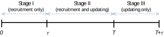
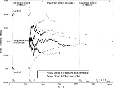
Figure 2:Optimal Bayes Sequential policy, together with four stage II/III paths of the posterior mean with prior meanµ0 ≈ 17. KEY: ‘*’ value of the sampling meanwi for each path i; ‘—-’ path of posterior mean when in stage II; ‘_{· · ·}’ path of posterior mean when in stage III. ‘+’ thresholds A, B, C, D delineate the ranges for ‘no trial’/‘fixed trial’/‘sequential trial recruitment’; ‘_◦’ optimal stage I sample sizes.

Figure 2 plots the optimal stopping boundaries in (n0 +t)× prior/posterior mean space, together with some stage I optimal sample sizes and four stage II/III paths of the posterior mean. The boundaries between the ‘no trial’/‘fixed trial’/‘sequential trial recruitment’ ranges for the prior mean are marked with a ‘+’ and labelled A, B, C and D. If the prior mean is above A or below B, it is optimal not to carry out any trial and instead base the technology adoption decision on the value ofµ0 alone. If the prior mean is between A and C or D and B, it is optimal to carry out a fixed sample trial (do stage I sampling and continue to stage III, with no stage II sampling). The optimal fixed sample sizes for such trials for some values of the prior mean are indicated by ‘_◦’ in these two regions. Ifµ0 lies between C and D, it is optimal to carry out a sequential trial, with stage II sampling. The stage II free boundaries are shown as dashed lines.

Figure 2 shows that stage II starts at an effective sample size of n0 +τ = 1100 pairwise allocations. Because there is no discounting, there is symmetry above and belowµ= I/P = 0 in the stage II stopping boundary and the stage I fixed sample sizes (recall Prop. 2.4).

of theXifori= 1,2, . . .given that draw, to generate the sample pathµtusing Eqs. (2) and (3b). Figure 2 shows four sample paths for a prior mean of µ0 ≈ 17 lying in the ‘sequential trial recruitment’ region, meaning that it is optimal to proceed to stage II. The realised values ofWi, i = 1,. . . ,4 are indicted by ‘*’s. Stage II sections of the paths are marked as continuous lines. When a stage II path first touches the upper or lower stage II stopping boundary (dashed line), it is optimal to proceed to stage III, at which point the paths are shown as dotted lines. For path 1, w1 >0 and the path crosses the upper stopping boundary soon after entering stage II. The new technology is selected upon the conclusion of stage III, because the posterior mean is positive. This is the correct decision, given thatw1 > 0. The same applies for path 2, with the posterior mean hitting the upper boundary a little later than for path 1. For path 3, w3 < 0 and the new technology is rejected once all pipeline subjects have been observed (again the correct decision). Path 4 results in an incorrect decision: w4 > 0, but the path exits stage II close toTmax (on the lower free boundary) and, upon conclusion of stage III, the new technology is rejected because the posterior mean is negative after all pipeline subjects have been observed.

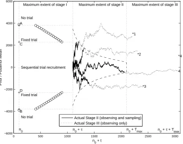
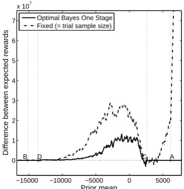
Figure 3(a) plots the difference between the averages of the realised rewards obtained from the Optimal Bayes Sequential policy and those from the two alternative policies: the ‘Fixed’ policy, which always makesTmax=2000 pairwise allocations, and the Optimal Bayes One Stage policy of Eq. (14). Thick lines represent the averages, dotted lines 95% confidence intervals. For convenience, we call this difference the ‘net gain’. Figure 3(b) shows the proportion of iterations which make the correct adoption decision. To derive each graph, we chose 400 equally-spaced values ofµ0in the range[-6000,6000]and, for each value ofµ0, the results from 15,000 sample paths were averaged.1

Figure 3(a) shows that, as expected, the Optimal Bayes Sequential policy outperforms the other two policies when judged according to net gain. Compared with the ‘Fixed’ policy, the greatest gains for the Optimal Bayes Sequential policy may be seen at extreme values of the prior mean, which is unsurprising: there is little point running a trial with a large fixed sample size when the prior mean is far from zero. The net gain is lowest aroundµ0 =I/P (= 0). These findings are reversed for the Optimal Bayes One Stage policy, which yields an optimal sample size equal to that of the Optimal Bayes Sequential policy to the left of D and to the right of C, so that there is no difference between the expected rewards. Between D and C, the Optimal Bayes Sequential policy benefits from the arrival of observations on the pipeline subjects to update the prior distribution and offers the flexibility to stop stage II according to the value of the posterior mean and variance. No such luxury is available for the other policies, which commit to sampling and observing a predetermined number of observations regardless of the information that arrives. Figure 3(b) plots the estimate of the probability that each of the three sampling policies correctly selects the best technology. The probabilities for the Optimal Bayes Sequential policy and the Optimal Bayes One Stage policy coincide to the left of D and the right of C for the reasons just stated. Between D and C, the Optimal Bayes Sequential policy is superior because its decision rule sequentially updates the information after each observation. The Fixed policy performs best for the probability of correct selection because it guarantees the highest amount of

1_{Smooth curves in the paper are obtained from the partial differential equation methods of Appendix S. The}

−6000−2 −4000 −2000 0 2000 4000 6000 0

2 4 6 8 10x 10

5

Prior mean

Difference between expected rewards

A

B D C

Optimal Bayes One Stage Fixed

(a) ‘Net gain’ in expected reward of Optimal Bayes Sequential over comparator policies.

−60000.9 −4000 −2000 0 2000 4000 6000 0.91

0.92 0.93 0.94 0.95 0.96 0.97 0.98 0.99 1

Prior mean

Proportion of correct decisions

A

B D C

Optimal Bayes Sequential Fixed

Optimal Bayes One Stage

(b) Proportion of simulations which make the cor-rect adoption decision.

Figure 3:Operating characteristics for the illustration of section 3.

information. This is obtained at an economic cost, however (refer to Figure 3(a)).

In section S.6.1 we illustrate the effect of reducing the delay fromτ = 1000 to 500 pairwise allocations. Stage II boundaries change shape slightly but are shifted left (τ is smaller). There are no stage I optimal sample sizes (point D moves to point B, and point C moves to point A).

4

Unknown sampling variance

The analysis to date has assumed that the sampling variance,σ2

X, is known, but in practice this will not be the case. This section extends the analysis to the case whenσ2

X is unknown, adopting and developing the framework proposed by Chick et al. (2015).

DefineTν as a standard Studenttrandom variable withνdegrees of freedom (dof) and define φν andΦν as, respectively, its pdf and cdf. Denote the distribution of the three parameter Student trandom variable,µ+Tν/√κ, asSt(µ, κ, ν)_{, with precision}κ_{. If}ν > _2,Var[Tν] =ν/(ν−₂)_. As before, assume thatXi are normally distributed and conditionally independent, given the unknown expected value,W, andunknownσ2

X. Letς be the random variable whose realization isσ2

X. We choose a prior distribution in the conjugate family for normally distributed samples with unknown mean,W, and variance,ς (DeGroot, 1970, § 9.6). Then:

Xi |W, ς iid∼ N(W, ς),

ς ∼ InvGamma_{(ξ0, χ0), (15)}

W|ς ∼ N(µ0, ς/η0),

andη0 determine the a priori mean and variance of the unknown sampling mean. It follows that W is aSt(µ₀, ξ₀η₀/χ₀,2ξ₀)_{random variable and}Var[W] =χ₀/[(ξ₀−₁)η₀]_whenξ₀ >_1.

Fort = 0,1, . . . , τ ₋1, no observations arrive owing to the delay, soξt+1 = ξt,χt+1 = χt,

ηt+1 = ηt, andµt+1 = µt. Fort = τ, τ +1, . . ., the posterior distribution can be updated by adapting DeGroot (1970) to account for observations on the pipeline subjects as follows:

ς_|Xt+1−τ,Ft ∼ InvGamma(ξt+1, χt+1),

W_|ς, Xt+1−τ,Ft ∼ N(µt+1, ς/ηt+1),

W| Ft ∼ St(µt, ηtξt/χt,2ξt),

where ξt+1 = ξt +1/2, χt+1 = χt + _2(ηtηt₊₁₎(µt − Xt+1−τ)2, ηt+1 = ηt +1, and µt+1 = (ηtµt+Xt+1−τ)/ηt+1. We note thatξt andηtare deterministic functions of t, given ξ0 andη0. The posterior precision,ξtηt/χt, is the Bayesian analog of the frequentist observed information I(t−τ)+ given(t−τ)+observations (Hampson and Jennison, 2013, § 6 on unknown variance).

The predictive distribution for the posterior mean given that sampling stops at time T = t, with state(µt, χt, t), and withu= min(T, τ)pipeline subjects to arrive, is (DeGroot, 1970):

Zt,u _∼St

µt,ξtηt

χt

(ηt+u)

u ,2ξt

(16)

(compare with Eq. (6) for the case of known variance). Just as for the case of knownσ2

X, the optimal solution involves solving stages I, II and III as illustrated in Figure 1. In contrast to the case of knownσ2

X, the state vector(µt, χt, t), and not

(µt, t), is sufficient to summarize_Ftfor the purposes of inference about W. Stages I and III are

straightforward to modify: the stage III terminal reward function in Eq. (7) is modified by taking the expectation in its RHS with respect to the Student t distribution forZt,u in Eq. (16), rather than the normal distribution of Eq. (6). A similar change is sufficient to modify the expectation in the RHS of Eq. (14) for stage I, to determine the Optimal Bayes One Stage policy.

Chick et al. (2015) proposed three approaches to solving stage II for the case of unknownσ2

X.

Here we extend the so-calledKG∗ variant of the knowledge gradient (Chick and Frazier, 2009; Frazier and Powell, 2010) which, given information to hand, continues sampling if and only if there exists a feasible one-stage sampling policy giving a greater expected reward than would be gained from stopping.

DefineBβˆ (µt, χt, t)to be the expected value of making β ≥ 0more pairwise allocations at timet, observing the remainingβ+ min(t, τ)outcomes, accruing online rewards (if applicable), and selecting the better technology:

ˆ

Bβ(µt, χt, t) = E

β−1

X

i=0

−c+δonXt+i+1 (1 + ˜ρ)i

+(P Z

′

t,β+min(t,τ)−I)+ (1 + ˜ρ)1β+t>0(β+τ)

Ft

. (17)

whereZ′

To adapt stage II to the case of unknown sampling variance, we replace the value of continu-ing over all nonanticipative policies (the second term in the maximand of Eq. (8a)) with a set of one-step lookahead policies,_Bt. Thus, Eq. (8a) is approximated by

ˆ

B∗_(µ

t, χt, t) = max

ˆ

B0(µt, χt, t),max

β∈Bt

ˆ

Bβ(µt, χt, t)

, t_∈T_{II. (18)}

The set_Bt ={1,2, . . . , Tmax−t}contains the nonzero pairwise allocations which remain. The choice_Bt = {2−1/2,1,21/2, . . . ,min(128, Tmax−t)}proved useful as an approximation and is used in numerical results here. Letβ∗ _{= arg max}

β∈BtBβˆ (µt, χt, t).

We define theKG∗ continuation setCKG∗ here to be the set of(µt, χt, t)such that one

con-tinues to allocate if and only if Bβˆ ∗(µt, χt, t) > Bˆ₀(µt, χt, t)(i.e., there is a non-zero, feasible

one stage sampling plan whose expected reward exceeds that of stopping immediately and acting optimally once the observations on the pipeline subjects are observed).

A second approach to solving stage II that was proposed by Chick et al. (2015) is based on the numerical solution of the PDE free boundary problem. This adjusts the variance of the diffusion process to account for the uncertainty on σ2

X and is briefly described in Appendix S.6.3. The following application considers the operating characteristics of both approaches to dealing with an unknown sampling variance.

5

Application: drug-eluting stents

Moses et al. (2003) and Cohen et al. (2004) compared the performance of drug-eluting stents (DES, the new technology) with bare metal stents (BMS, the standard) for the treatment of com-plex coronary stenoses using percutaneous coronary intervention (PCI) in the ‘SIRIUS’ trial. The authors randomised 1058 patients to either DES or BMS and measured clinical outcomes, resource use and costs over a one year follow-up period. The trial’s recruitment phase lasted approximately seven months, so it did not include a period during which observations on the primary end points were being made while recruitment was taking place.

We consider the performance of the Optimal Bayes Sequential policy of section 2 (known sampling variance) and the policy of section 4 (unknown sampling variance) with what is a Fixed policy with the same sample size as the SIRIUS study (529 patient pairs in 7 months) and the Optimal Bayes One Stage policy. For the purposes of this section, we setδCE = 1in Eq. (1) to concentrate on the cost and QALY results at one year of follow-up that are reported in Cohen et al. (2004). This section is intended to illustrate how our model may be populated with data from a health technology assessment; it is not intended to represent a comment on the health technology itself.

5.1 Known sampling variance

Where possible, parameter values are derived from Moses et al. (2003) and Cohen et al. (2004).

Otherwise they are based on assumptions. The value of σX = $17358 is derived from point

0 500 1000 1500 2000 2500 −15000 −10000 −5000 0 5000

Prior / Posterior Mean

n

0 + t

n

0 n0 + τ n0 + Tmax

No trial No trial Sequential trial recruitment A B C D

(a) Optimal Bayes Sequential policy.

−15000 −10000 −5000 0 5000 0 1 2 3 4 5 6 7

x 107

Prior mean

Difference between expected rewards

A

B D C

Optimal Bayes One Stage Fixed (= trial sample size)

(b) ‘Net gain’ in expected reward of Optimal Bayes Sequential over comparator policies.

−15000 −10000 −5000 0 5000 0 200 400 600 800 1000 1200 1400 1600 1800 2000 2200 Prior mean

Expected sample size

A

B D C

Optimal Bayes Sequential Fixed (= trial sample size) Optimal Bayes One Stage

(c) Expected sample size.

−15000 −10000 −5000 0 5000 0.9 0.91 0.92 0.93 0.94 0.95 0.96 0.97 0.98 0.99 1 Prior mean

Proportion of correct decisions

A

B D C

Optimal Bayes Sequential Fixed (= trial sample size) Optimal Bayes One Stage

(d) Proportion of simulations which make the cor-rect adoption decision.

Figure 4: Optimal Bayes Sequential policy and operating characteristics for the stents application of sec-tion 5 (known variance).

which is higher than the annual rate of recruitment to the study (calculated to be R = 529_× 12/7 = 907 patient pairs per year). The delay in response is one year, so τ = 907. A zero switching cost is assumed (I = 0) and the effective sample size in the prior distribution is assumed to ben0 = 20. We assumec = $200 andP = 2×106. In contrast to the illustration of section 3, the discount rate is chosen to be 1% per annum (ρ˜= (1 + 0.01)−R_{−1). Benefits} accruing to trial participants are not valued (δon =0).

sample size that is neither too close to 0, nor too close toτ. This is because, at points A and B, the expected value of taking a small, fixed, sample size is more than offset by the cost of postponing the adoption decision that is implied by starting to experiment (by experimenting, one must wait for at least a year before making the adoption decision, and rewards are discounted). For a prior mean lying between points C and D it is optimal to proceed to stage II.

In the absence of discounting, Prop. 2.4 implies that there is a greater expected reward when the posterior mean is above I/P = 0 than when it is below that value by the same absolute amount. With a positive discount rate, the expected benefit of continued sampling is penalized more for values of the posterior mean aboveI/P than for values below it by the same absolute amount. Consequently, the upper stage II boundary in Figure 4(a) is shifted down relative to the upper stage II boundary for the case of zero discounting (latter not shown). The change is greater in magnitude than the corresponding change for the lower boundary, resulting in asymmetric stopping boundaries for a positive discount rate.

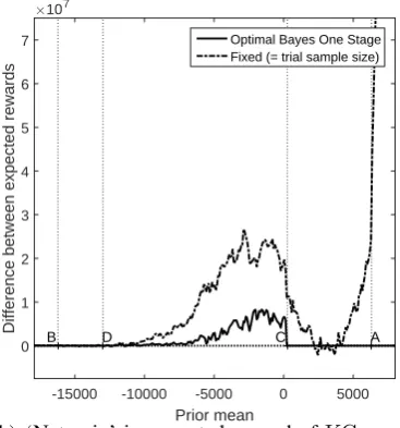
This asymmetry is reflected in the plots of the ‘net gains’ (the differences between the ex-pected reward of the Optimal Bayes Sequential policy and the two comparators) in Figure 4(b) and the expected sample sizes in Figure 4(c). In Figure 4(b), the negative values (indicating that the Optimal Bayes Sequential policy performs less well than its comparator) close to point C are due to the noise in the Monte Carlo estimates and the fact that the expected sample sizes of the three comparators are quite close to each other in the vicinity of point C (Figure 4(c)). Figure 4(c) also illustrates the ‘jumps’ in the expected sample sizes for the different trial designs at points A–D (see the discussion of Figure 4(a) above).

For a value of the prior mean close to zero, Figure 4(b) shows that the expected net gain of the Optimal Bayes Sequential policy over the Fixed policy is approximately $20m and over the Optimal Bayes One Stage policy it is $10m. Not apparent from Figure 4(b), due to the scaling, is that fact that, for extremely low values of the prior mean, the difference in rewards between the Optimal Bayes Sequential policy and the Fixed policy converges to a positive value equal to the discounted cost of sampling patients under the Fixed policy. This is because, if the value of the prior mean is low enough, it will be optimal not to start the trial under the Optimal Bayes Sequential policy, whereas the Fixed policy will always make 529 pairwise allocations and then reject the new technology with very high probability. Asµ0 → ∞, the net gain of the Optimal Bayes Sequential policy over the Fixed policy grows without bound: with a very optimistic prior mean, it is optimal to adopt immediately under the Optimal Bayes Sequential policy, whereas the Fixed policy is committed to incurring trial costs and discounting rewards.

−15000 −10000 −5000 0 5000 −0.5

0 0.5 1 1.5 2 2.5 3 3.5x 10

7

Prior mean

Reward: Optimal Bayes vs. Bayes One Stage

recr. rate: 907 per y. ( τ=907) recr. rate: 680 per y. ( τ=680) recr. rate: 453 per y. ( τ=453)

(a) Difference between expected reward of Optimal Bayes Sequential and Optimal Bayes One Stage poli-cies for several recruitment rates.

−15000 −10000 −5000 0 5000 0

1 2 3 4 5 6 7 8x 10

6

Prior mean

Difference in value at t=0

recr. rate: 680 per y. ( τ=680) recr. rate: 453 per y. ( τ=453)

(b) Expected reward of Optimal Bayes Sequen-tial policy: expected reward when recruitment rate is 907/year minus expected reward when it is 680/year and 453/year.

Figure 5:Effect of changingτ by changing the recruitment rate.

shown in Figure 4(d). This shows that the Optimal Bayes Sequential policy is superior to both the Fixed and the Optimal Bayes One Stage policies in the region DC, where the probability of selecting correctly is no lower than 0.96. It is similar to the comparators to the left of D. Over the majority of the range CA, the Fixed policy performs best because it tends to sample more (Figure 4(c)). Figure 4(d) shows that the proportion of correct decisions for the Optimal Bayes Sequential policy drops at points C and A. These drops mirror the jumps in the expected sample sizes that occur at those points (Figure 4(c)).

The estimate of the probability of a ‘decision reversal’ (the probability that the adoption decision that would have been made at the time of stopping to sample sequentially is overturned once all realisations on pipeline subjects have arrived) did not exceed 0.03 in this application.

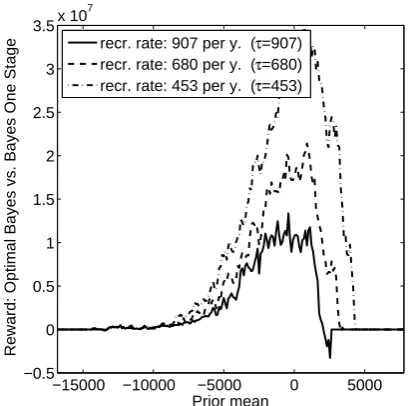
Figure 5(b) focuses on the Optimal Bayes Sequential policy showing that, for this application, the higher is the recruitment rate, the higher is the expected reward.

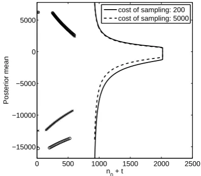
Figure 8 of Appendix S.6.2 shows the impact of changing the recruitment rate on the expected sample size. Figure 9 shows the stopping boundaries for different values of the sampling costc.

5.2 Unknown sampling variance

When the sampling variance is unknown, the following additional parameters are required to implement the model of section 4. For the prior distributions, we setη0 = n0 (η0 and n0 both represent the sample size in the prior distribution for the unknown mean), ξ0 = 2n0 − 1 and χ0 = 173582(ξ0 −1), so that E[ς] equals the point estimate of the sampling variance (σ2X = 173582) from the study. The KG∗ continuation set isestablished for the value of χt such that

χt/ξtequals 173582. The continuation set for otherχtcan be found by rescaling states (namely,

(µt, χt, t)∈ CKG∗ if and only if(aµt, a

2_{χt, t)∈ C}

KG∗).

Figure 6 replicates Figure 4 for the case of unknown variance, solved usingKG∗. A compar-ison of Figure 6(a) with Figure 4(a) shows that the continuation set of Stage I is slightly wider when the variance is unknown, owing to the additional dimension of uncertainty. The opposite effect is seen in Stage II, because theKG∗ approach is one stage and so the value of continuing is lower than the fully sequential approach adopted for the case of known variance. As a result, the expected sample size is smaller forKG∗ (Figures 6(c) and 4(c)) owing to earlier stopping, on average, and there is a smaller advantage in terms of the proportion of correct decisions (Fig-ures 6(d) and 4(d)). This, in turn, implies that the net gain in comparison with alternative policies is slightly reduced (Figures 6(b) and 4(b)).

Section S.6 of the OSM discusses the results obtained by replacing theKG∗ approach with one based on the numerical solution of the PDE free boundary problem and plug-in estimates of the sampling variance (Chick et al., 2015). The net gain (Figure 10) is very similar to the case of known variance.

The results of additional simulations (data not shown) suggest that the advantage of the Op-timal Bayes Sequential Policy over a Fixed Policy remains whenρ˜is smaller. Those results also show that the benefit of the Optimal Bayes Sequential Policy over the Optimal Bayes One Stage policy decreases asρ˜decreases.

6

Discussion

0 500 1000 1500 2000 2500

n₀ + t

-15000 -10000 -5000 0 5000

Prior / Posterior Mean

n

0 n0 + τ n0 + Tmax

A

B C

D

(a) Stopping boundary withKG∗ approach in sec-tion 5.2.

-15000 -10000 -5000 0 5000

Prior mean 0 1 2 3 4 5 6 7

Difference between expected rewards

×107

A

B D C

Optimal Bayes One Stage Fixed (= trial sample size)

(b) ‘Net gain’ in expected reward of KG∗ ap-proach over comparator policies.

-15000 -10000 -5000 0 5000

Prior mean 0 200 400 600 800 1000 1200 1400 1600 1800 2000 2200

Expected sample size

A

B D C

Optimal Bayes Sequential Fixed (= trial sample size) Optimal Bayes One Stage

(c) Expected sample size.

-15000 -10000 -5000 0 5000

Prior mean 0.9 0.91 0.92 0.93 0.94 0.95 0.96 0.97 0.98 0.99 1

Proportion of correct decisions

A

B D C

Optimal Bayes Sequential Fixed (= trial sample size) Optimal Bayes One Stage

(d) Proportion of simulations which make the cor-rect adoption decision.

Figure 6:Operating characteristics for the stents application of section 5 withKG∗approach in section 5.2 to approximate Optimal Bayes Sequential policy with unknown sampling variance.

the presence of delay in observing the primary end point? How do parameters such as the rate of patient recruitment and the cost of sampling influence optimal design?

the expected sample size is close to, or greater than, the expected sample sizes of those policies. Further, the higher is the delay, the less attractive is the sequential design over the Fixed and the Optimal Bayes One Stage policies. Clearly, the precise performance of the model will depend on the particular application of interest.

Directions for future research are numerous. The model assumes that only two health tech-nologies are being considered, it does not incorporate intermediate outcomes that are correlated with the primary end point and it is assumed that all pipeline data must be observed before an adoption decision is made. Future work includes relaxing these assumptions and exploring further the issues of unknown sampling variance and sensitivity of the policy to the choice of sampling distribution.

A

Mathematical proofs for the discrete time model

Proof of Prop. 2.1. Condition onW andT in Eq. (4) and use the tower property of conditional expectation:

Vπ(µ0, n0) = Eπ

Ehn

T−1

X

t=0

−c+δonXt+1 (1 + ˜ρ)t

o

+ 1D=N(P W −I) (1 + ˜ρ)1T >0(T+τ)

W, T i

µ0, n0

=E_π

nT_X−1

t=0

−c+δonW

(1 + ˜ρ)t

o

+ 1D=N(P W −I) (1 + ˜ρ)1T >0(T+τ)

µ0, n0

. (19)

Substituting Eq. (12) into the RHS of Eq. (11) and simplifying gives Eq. (19). _Kπ ≥ 0 when δon = 0 becausec≥ 0. Whenδon = 1it is strictly positive forW < cand 0 otherwise. Sπ ≥ 0 because (W ₋c)+ _{≥ 0. ρ˜ ≥ 0, τ ≥ 0, T ≥ 0 imply that(1 + ˜ρ)}1T >0(T+τ) ≥ 1_{. Further,}

(P W ₋I)+ _{≥ 0 and (P W −I)}+ _≥

1D=N(P W −I). Hence, (P W −I)+ ≥ 1D=N(P W −

I)/(1 + ˜ρ)1T >0(T+τ)independent of the sign of₁

D=N(P W −I). Thus,Lπ ≥0.

Proof of Prop. 2.2. From Eq. (11), a policy π in a given set of policies maximises Vπ _if and only if it minimises V˜π_{. This reformulation is useful, because the non-negativity of K}

π,t,

Sπ andLπ for all(yt, t, W)satisfies the (F+) property of Bertsekas and Shreve (1978, Chap. 8, p. 192). However, Bertsekas and Shreve (1978, Chap. 8) require rewards which depend on a known state vector, whereas_Kπ,t, Sπ, and Lπ depend on the unknownW. Following Bertsekas (2005, p. 218-222), we augment the state to be(yt, t, W), define the information vectorIt with

I0 = (0, y0)and It = (t, y0, y1, . . . , yt, a0, . . . , at−1)fort = T\{Tmax}, and must now allow a

broader set of policiesπ˜whose actionsatmay depend onIt, not just(yt, t).

Call the problem of finding a policy π˜ to minimize V˜π˜_{, the ‘regret problem.’ Its Bellman} equation, B˜(yt, t, W), consists of minimizing the expected cost of stopping (the first time at whichat= 0),

E

"

−G(yt, t) + (P W ₋I)++

Tmax−t−1

X

t=0

δon(W −c)+/(1 + ˜ρ)t | It #

and of making an additional pairwise allocation and proceeding optimally thereafter (at = 1),

E_{[c−δon(W −(W −c)}+_{) + (1−(1 + ˜ρ)}−1_{)(P W −I)}+

+ (1 + ˜ρ)−1B˜(yt+1t≥τXt+1−τ, t+ 1, W) | It], (21)

fort =T_{\{Tmax}. Its terminal cost isB}˜_{(yTmax, Tmax, W) =G(yTmax, Tmax).}

Because the (F+) property holds for this problem, Prop 8.1 and Cor. 8.1.1 of Bertsekas and Shreve (1978) justify that it suffices to consider nonrandomised Markovian policies within the set of all policies when solving infπ˜V˜˜π. Let π˜_B˜ be determined by B˜ for the regret problem. Although π˜_B˜ may depend on It for decisions at, note that (yt, t) is sufficient for W: π˜_B˜ is Markovian in(yt, t). Props. 8.2 and 8.5 of Bertsekas and Shreve (1978) show thatπ˜_B˜ is optimal, that is,V˜π˜_B˜_(µ

0, n0) = ˜B(µ0n0,0, W) = infπ˜V˜π˜(µ0, n0).

The expectations in B˜ depend on It only through (yt, t), and π˜_B˜ is therefore feasible for the original problem. By Prop. 2.1,π˜_B˜ is optimal for the original problem, andVπ˜B˜(µ₀, n₀) =

Vπ∗

(µ0, n0) = ¯V(µ0, n0)−B˜(µ0n0,0, W).

To complete the proof, we show that π˜_B˜ also satisfies Bellman’s equation of the original problem. By definition, π˜_B˜ chooses the smaller of Eq. (20) and Eq. (21). It therefore makes the same choices if one subtracts the same quantity from both equations. In particular, π˜_B˜ is still optimal if one subtractsE_{[(P W −I)}+₊PTmax−t−1

t=0 δon(W −c)+/(1 + ˜ρ)t| It]from both Eq. (20) and Eq. (21). With a bit of algebra, one confirms that these subtractions result in terms which, in expectation, are -1 times the maximands in Bellman’s equation, Eq. (8) and Eq. (9), for the original problem. Because₋min(−a,−b) = max(a, b),π˜_B˜also satisfies Bellman’s equation of the original problem. Setting t = 0in the subtracted terms allows us to show B(µ0n0,0) =

¯

V(µ0, n0)−B˜(µ0n0,0, W). ThusB(µ0n0,0) =Vπ

∗

(µ0, n0).

Proof of Prop. 2.3. The proof is like that of Prop. 2.2, except that the infinite horizon re-sults of Bertsekas and Shreve (1978, Chapter 9) are employed. Because_Kπ, Sπ, andLπ are all nonnegative, the (P) assumption of Bertsekas and Shreve (1978, page 214) is satisfied for the minimisation of the expectation of _Kπ +Sπ +Lπ. The (P) assumption is the infinite horizon analog of the (F+_{) property for the finite horizon. Because of the Markovian nature of Bayes’} rule, Bertsekas and Shreve (1978, Prop. 9.1) show that an additional dependence of the state evo-lution on the past can not bring additional expected reward. Bertsekas and Shreve (1978, Prop. 9.8) justify the claim that the value function in Eq. (5) satisfies Bellman’s equation for the regret problem, V˜˜π_B˜(µ

0, n0) = ¯B(µ0n0,0), and V˜π˜B˜(µ₀, n₀) = ˜Vπ∗(µ₀, n₀) follows from Bertsekas and Shreve (1978, Prop. 9.12). The link fromV˜ back toV is as for Prop. 2.2.

Proof of Prop. 2.4. We first prove claim (ii), that B((I/P + ∆µ)nt, t) = B((I/P −

∆µ)nt, t)₋P∆µfor t = 0,1, . . . , Tmax, in two steps: we show that the first term in the

max-imand of Eq. (8a), G(_·), satisfies a similar relation involving∆µfor allt, so that B(_·)satisfies the claimed relationship whent =Tmax. Then an induction argument in−twill prove the result

fort = 0,1, . . . , Tmax−1. Claims (i) and (iii) will follow from the proof of claim (ii).

of a standard normal random variable (DeGroot, 1970). Moreover,

E_[(−Z)+_{] =σ[φ(−ξ}′_)−ξ′_Φ(−ξ′_{)] =σ[φ(ξ}′_{) +ξ}′_Φ(ξ′_{)]−ξ. (22)}

Consider an arbitrary state, (µt, t), and pick ∆µ so that µt = I/P + ∆µ. Then P µt = I +P∆µ and yt = (I/P + ∆µ)nt. We define some additional notation to help us proceed. Define µt˜ = I/P ₋ ∆µ, so that Pµt˜ = I ₋ P∆µ and yt˜ = (I/P ₋∆µ)nt. Recall that, given information to time t, ZT,min(T,τ) has mean µt = yt/nt. LetZT,˜ min(T,τ) be the predictive distribution for the posterior mean given stopping at timetwithYt = ˜yt. Then:

E_{[P ZT,min(T,τ)−I |YT =yt, T =t] =P∆µ, (23a)}

E_[PZT,˜ _{min(T,τ)−I |YT =yt, T =t] = −P∆µ. (23b)}

Defineσ2 _{= Var[(P ZT,}

min(T,τ)−I)|YT, T =t], which depends ontbut not onYT. Given the assumptionρ˜= 0, we may simplify Eq. (7) using Eqs. (23a) and (23b):

G(yt, t) =E_{[(P ZT,min(T,τ)−I)}+ _{|YT =yt, T =t]}

=σ[φ(P∆µ/σ) + (P∆µ/σ)Φ(P∆µ/σ)]

=σ[φ(₋P∆µ/σ) + (₋P∆µ/σ)Φ(₋P∆µ/σ)]₋(₋P∆µ)

=E_{[P( ˜ZT,min(T,τ)−I/P)}+_{|YT = ˜yt, T =t] +P∆µ}

=G(˜yt, t) +P∆µ. (24)

Thus, given Eq. (8b),B(yt, t)₋P∆µ=B(˜yt, t)fort=Tmax.

Suppose now thatB(yt+1, t+1)−P∆µ=B(˜yt+1, t+1)for somet ∈ {τ, τ+1, . . . , Tmax−1}, so that the claimed relation holds at timet+ 1. We now show that this relation holds at timetby proving a similar relation for each maximand which determinesB(_·).

By Eq. (24), the first maximand on the right hand side of Eq. (8a) differs by P∆µ when evaluated atyt = (I/P + ∆µ)nt andy˜t = (I/P −∆µ)nt, as desired. Let B2 be the second maximand in the right hand side of Eq. (8a). Ift _≥ τ, letXˆ be a normal random variable with mean 0 and varianceσ2

X. Ifδon = 0andρ˜= 0then

B2(yt, t)−B2(˜yt, t) = Eπ[B(yt+yt/nt+ (Xt+1−τ −yt/nt), t+ 1)|YT =yt, T =t]

−E_{π[B(˜yt+ ˜yt/nt+ (Xt+1−τ −y˜t/nt), t+ 1)|YT = ˜yt, T =t]}

= E_{[B(yt+yt/nt+ ˆX, t+ 1)|YT =yt, T =t]}

−E_{[B(˜yt+ ˜yt/nt−X}ˆ_{), t+ 1)|YT = ˜yt, T =t] (25)}

= E_{[P(∆µ+ ˆX/nt+1)|YT =yt, T =t] =P∆µ. (26)}

Ift < τ, then it is straightforward to show thatB2(yt, t)−B2(˜yt, t) =P∆µfrom Eq. (9). By mathematical induction,B(yt, t)−P∆µ=B(˜yt, t)fort=Tmax, Tmax−1, . . . ,1,0. This justifies claim (ii). By settingt= 0and by recalling Eq. (13), we obtainVπ∗

(I/P + ∆µ, n0)−

P∆µ=Vπ∗

(I/P −∆µ, n0). This justifies claim (i).

We have shown (a) that the first maximand differs by the same amount (by ₋P∆µ) when evaluated at(yt, t)and(˜yt, t), and (b) that the second maximand in Eq. (8a) differs by the same amount (by ₋P∆µ) when evaluated at (yt, t) and (˜yt, t). Thus, either the first maximand is larger for both(yt, t)and(˜yt, t)or the second maximand is not smaller for both(yt, t)and(˜yt, t). Recall that(yt, t)and(˜yt, t)correspond to the points(µt, t)and(˜µt, t), respectively. This relation among the maximands implies that(µt, t)is in the interior of the continuation set when(˜µt, t)is in the continuation set, and vice versa. This proves claim (iii).

Proof of Prop. 2.5. Follows directly from Chick and Frazier (2012, Prop. 3). See Ap-pendix S.1 in the OSM for further detail.

Acknowledgements

We thank participants in the 2014 annual conference of the Royal Statistical Society, Sheffield, the 2014 IDEAL (Integrated Design and Analysis of Clinical Trials) consortium Annual Scientific Meeting, Paris, and 2015 seminars at the Chicago Booth School of Business, INSEAD, the Yale School of Management, and Bocconi and Bologna Universities, as well as Noah Gans and Jacco Thijssen, for comments on earlier versions of this work. Priming monies came from fund RIS6.1(2013–2014) of the Department of Economics and Related Studies, University of York. The usual disclaimer applies.

References

Armitage, P. (1975).Sequential Medical Trials. Blackwell Oxford.

Berry, D. A. (1985). Interim analyses in clinical trials: classical vs. Bayesian approaches. Statistics in Medicine, 4:521–526.

Berry, D. A. and Ho, C. (1988). One-sided sequential stopping boundaries for clinical trials: a decision-theoretic approach.Biometrics, 44:219–227.

Bertsekas, D. and Shreve, S. (1978). Stochastic Optimal Control: The Discrete Time Case. Academic Press, Belmont, MA.

Bertsekas, D. P. (2005). Dynamic Programming and Stochastic Control: Volume I. Athena Scientific, Belmont, MA, 3 edition.

Broglio, K. R., Connor, J. T., and Berry, S. M. (2014). Not too big, not too small: a Goldilocks approach to sample size selection.Journal of Biopharmaceutical Statistics, 24(3):685–705.

Brown, J., McElvenny, D., Nixon, J., Bainbridge, J., and Mason, S. (2000). Some practical issues in the design, monitoring and analysis of a sequential randomized trial in pressure sore prevention. Statistics in Medicine, 19:3389–3400.

Burman, C.-F. (2013). Discussion of the paper by Hampson and Jennison. JRSS, Series B, 75(1):47.