This is a repository copy of
Mean field electrodynamics: triumphs and tribulations
.
White Rose Research Online URL for this paper:
http://eprints.whiterose.ac.uk/133497/
Version: Accepted Version
Article:
Hughes, DW orcid.org/0000-0002-8004-8631 (2018) Mean field electrodynamics: triumphs
and tribulations. Journal of Plasma Physics, 84 (4). 735840407. ISSN 0022-3778
https://doi.org/10.1017/S0022377818000855
© 2018, Cambridge University Press. This article has been published in a revised form in
Journal of Plasma Physics [https:// doi.org/10.1017/S0022377818000855]. This version is
free to view and download for private research and study only. Not for re-distribution,
re-sale or use in derivative works. Uploaded in accordance with the publisher's
self-archiving policy.
eprints@whiterose.ac.uk https://eprints.whiterose.ac.uk/ Reuse
Items deposited in White Rose Research Online are protected by copyright, with all rights reserved unless indicated otherwise. They may be downloaded and/or printed for private study, or other acts as permitted by national copyright laws. The publisher or other rights holders may allow further reproduction and re-use of the full text version. This is indicated by the licence information on the White Rose Research Online record for the item.
Takedown
If you consider content in White Rose Research Online to be in breach of UK law, please notify us by
Mean Field Electrodynamics: Triumphs and
Tribulations
David W. Hughes
1†
1
Department of Applied Mathematics, University of Leeds, Leeds LS2 9JT, UK
(Received xx; revised xx; accepted xx)
The theory of mean field electrodynamics, now celebrating its fiftieth birthday, has had a profound influence on our modelling of cosmical dynamos, greatly enhancing our understanding of how such dynamos may operate. Here I discuss some of its undoubted triumphs, but also some of the problems that can arise in a mean field approach to dynamos in fluids (or plasmas) that are both highly turbulent and also extremely good electrical conductors, as found in all astrophysical settings.
1. The Need for a Mean Field Dynamo Theory
The origins of dynamo theory, and indeed one might argue the origins of magnetohy-drodynamics (MHD) itself, might be traced to the short, but hugely influential paper by Larmor (1919), entitled ‘How could a rotating body such as the Sun become a magnet?’, in which he postulated that the swirling motions inside stars could maintain a magnetic field. Theoretical progress following this paper was, however, not swift, and indeed the first concrete result in what we would now call dynamo theory was a negative one — the celebrated anti-dynamo theorem of Cowling (1933), showing that an axisymmetric magnetic field could not be maintained by dynamo action. The first example of a working dynamo did not come until a quarter of a century later, with the paper by Herzenberg (1958) showing how a magnetic field could be maintained by two widely separated spherical rotors with inclined axes of rotation in an electrically conducting fluid otherwise at rest.
One of the most important and long-standing issues in astrophysical fluid dynamics is to explain the generation of global-scale magnetic fields; i.e. magnetic fields with a significant component on the scale of the body in question. In broad terms, one might think of a global-scale dynamo as a mechanism by which toroidal field is created from poloidal field whilst, conversely and simultaneously, the poloidal field is regenerated from the toroidal field. Whereas the winding up of poloidal field into toroidal field can be readily explained as a natural consequence of a differentially rotating flow, essentially by Alfv´en’s theorem, the closing of the ‘dynamo loop’ (i.e. the regeneration of poloidal from toroidal field) is much less straightforward. It is here that the power of mean field electrodynamics really comes into its own — what is problematic in the full (unaveraged) MHD equations emerges naturally in their mean field counterparts. (Herzenberg’s model was ingenious, but his choice of flow cleverly sidestepped this issue.)
The means by which poloidal field could be regenerated from toroidal field in a turbulent flow was first addressed by Parker (1955), in one of many striking contributions to astrophysics. Although different in style to later formulations of mean field electro-dynamics, this can be recognised as the first paper on what we would now call mean field dynamo theory. Parker’s crucial insight was to recognise that small-scale cyclonic
motions could raise and twist toroidal field, and that the subsequent coalescence of the field loops thus formed would lead to a large-scale poloidal component of the magnetic field. This led to the vital new ingredient of a source term for the poloidal field and, consequently, to the development of what we would now call an αω-dynamo, with its associated propagating dynamo waves.
The idea of encapsulating the large-scale influences of small-scale interactions was developed into a beautifully elegant theory by Steenbeck, Krause and R¨adler in a series of papers in the 1960s; these were translated into English by Roberts & Stix (1971), and the ideas contained therein were elucidated and developed further in the monographs by Moffatt (1978) and Krause & R¨adler (1980). It is on these papers, together with that of Parker (1955), that the edifice of mean field electrodynamics has been built over the past fifty years, and which has formed the framework for investigating dynamo action in astrophysical bodies.
In this paper I shall discuss some of the most important results that have arisen from mean field dynamo theory, but shall also point out some of the difficulties encountered in applying the theory to the high conductivity, turbulent regime applicable in astrophysics. In this necessarily somewhat brief review, I shall concentrate on the formulation and fundamental aspects of the theory; it is though, even within these confines, far from comprehensive. Furthermore, over the years, certain aspects of mean field electrody-namics have proved quite controversial; some of the views presented here are certainly subjective, and not all are universally accepted.
2. Mathematical Formulation of Mean Field Electrodynamics
2.1. Large- and small-scale dynamos
The aim of mean field electrodynamics is to address what might be termedlarge-scale
dynamos. Before considering the mathematical details of mean field dynamo theory, it is therefore worth discussing the classification of dynamos in terms of their spatial scale. Although any such classification is somewhat imprecise, it does nonetheless highlight some important considerations. Let us first consider the case where there is a fluid velocity, either laminar or turbulent, with a single well-defined characteristic length scale,
ℓosay. Then, in rather general terms, we might categorise a large-scale dynamo as one in
which there is a sizeable fraction of the magnetic energy at scales very large compared with ℓ0. A more precise, and more satisfactory, requirement for a dynamo to be large scale would be that the spectrum of magnetic energy has a local maximum at large scales (together with another at the scale of the flow). A small-scale dynamo may be defined as one for which all significant scales of the field are comparable with or smaller thanℓ0. A small-scale dynamo can be unequivocally defined, at least computationally or exper-imentally: if amplification of magnetic energy is found in a domain of sizeO(ℓ0) then the flow is acting as a small-scale dynamo. Things become less clear in extended domains. If the domain of a small-scale dynamo is extended, then the magnetic energy will, almost certainly, possess some large-scale component; however, unless this is pronounced, it seems reasonable to categorise such a dynamo as essentially small scale. The strictest definition of a large-scale dynamo would be one that succeeds in a large enough domain, but fails when the domain size is reduced toO(ℓ0).
component, manifested through its appearance at the surface as active regions; however, it is also the case that the Sun has a strong global-scale flow in the form of its differential rotation. Thus, with both field and flow on the largest scale available, it is hard to go beyond saying that this is a global-scale or system-size dynamo.
2.2. Deriving the mean field induction equation
Although there are important and controversial questions concerning the nonlinear (dynamical) aspects of mean field electrodynamics, which we shall discuss later, it is formally a linear (kinematic) theory; we shall therefore first consider its formulation via only the induction equation. Thus, in standard notation, under the simplifying assumption that the magnetic diffusivityη is uniform, we consider the equation
∂B
∂t =∇×(U×B) +η∇
2
B, (2.1)
where it is assumed that there is no influence of the magnetic field on the velocity. The exposition below follows closely that of Moffatt (1978), in which further details can be found.
The underlying assumption of mean field theory is that there is some sort of scale separation between large and small scales, and that one then studies the evolution of averaged (or mean) quantities, where the average (which we shall denote byh·i) is taken over some intermediate scale. Here we shall consider the separation to be in spatial scales, which is the most natural framework for applications of mean field theory to astrophysical bodies. The velocity and magnetic field may then be expressed in terms of large- and small-scale components (or mean and fluctuating components) as
U=U0+u, B=B0+b, (2.2)
withhbi=hui= 0.
The mean induction equation then takes the form
∂B0
∂t =∇×(U0×B0) +∇×E+η∇
2
B0, (2.3)
whereE, the mean electromotive force (e.m.f.), is defined by
E=hu×bi, (2.4)
thus representing the projection onto the large scale of the interactions between the small-scale velocity and small-small-scale magnetic field. It is the presence of the term involving the e.m.f. that sets the mean induction equation apart from its unaveraged counterpart. Since here we are interested particularly in the formulation and interpretation of mean field electrodynamics, we shall from now on ignore the influence of the mean flow, setting U0= 0. Interactions between the mean flow and mean magnetic field, although extremely important, as discussed in the introduction, are not germane to considerations of the mean e.m.f. Hence (2.3) simplifies to
∂B0
∂t =∇×E+η∇
2
B0. (2.5)
To make progress with the mean field approach, via equation (2.5), one has to express the mean e.m.f. in terms of only mean quantities — the closure problem of mean field MHD. The standard approach is to consider the evolution equation for the fluctuating field, formed by subtracting (2.5) from (2.1):
∂b
∂t =∇×(u×B0) +∇×G+η∇
2
whereG=u×b− hu×bi. Formally we may write (2.6) as
L(b) =∇×(u×B0), (2.7)
whereLis a linear operator. It is at this stage, in seeking to solve (2.7) forb, that we en-counter the first potential difficulty, one to which we shall return in§3.4, namely whether there are non-decaying solutions toL(b) = 0. However, if we make the assumption that all solutions of the homogeneous equation L(b) = 0 decay in time, then we can regard the right hand side of (2.7) as a source term for the fluctuating field. In this case, the linearity between band B0, and hence that between E and B0, suggests an expansion ofE in terms ofB0 and its derivatives. This is usually written as
Ei=αijB0j+βijk
∂B0j
∂xk
+· · ·, (2.8)
where the coefficientsαij,βijk, etc. are pseudo-tensors governed by the properties of the
velocity field u(x, t) (pseudo-tensors because E is a polar vector whereas B0 is axial). Substituting (2.8) into (2.3) yields the mean induction equation for the evolution ofB0, namely
∂B0i
∂t =ǫijk ∂ ∂xj
αklB0l+βklm
∂B0l
∂xm
+· · ·
+η∇2
B0i. (2.9)
It should be noted that in the ansatz (2.8), and hence also in the mean induction equation (2.9), although higher order terms are suggested, consideration is only ever given to the first two terms in the expansion; indeed, inclusion of higher order terms would lead to spatial derivatives of higher than second order in the mean induction equation, thus rendering it of a very different mathematical character to the unaveraged induction equation.
For general flows, lacking any symmetry, theαandβtensors can lead to a wide variety of quite complicated effects (see, for example, Krause & R¨adler 1980; Roberts 1994). In order to get to the very essence of the theory, it is though often instructive to consider the simplified case in which the flow is isotropic and in which the mean field tensors therefore simplify to αij = αδij, βijk = βǫijk, where α is a pseudo-scalar and β is a
pure tensor. With the further simplifying assumption that αand β are constants (i.e. not dependent on the large spatial scale), equation (2.9) simplifies to
∂B0
∂t =α∇×B0+β∇
2
B0, (2.10)
assuming β ≫ η. Whereas, in this simplest formulation, β is clearly an additional, turbulent, contribution to the magnetic diffusivity, the term involving α (the dynamo ‘α-effect’) is of a completely different character to the induction term in the unaveraged equation (2.1); the mean e.m.f. is parallel to the mean field, whereas the e.m.f. is orthogonal to the magnetic field. From (2.10), the growth rate p of a long wavelength perturbation with wavenumberkis then given by
p∼αk−βk2
. (2.11)
helicity, defined by
H=hu·∇×ui. (2.12)
It is thus easy to see, without looking too far, why helicity plays such a dominant role in mean field electrodynamics.
Finally in this sub-section we note that while the derivation of the mean field induction equation (2.9) is a consequence of an assumed separation of spatial scales, one might also consider the problem of dynamo action in a flow that has two very different temporal
scales. Interestingly, the mean induction equation, now depicting the evolution of the magnetic field on long timescales, takes a different form, as shown by Herreman & Lesaffre (2011) and Vladimirov (2012). Rather than the new mean field contribution being anα -effect, it instead takes the form of an additional Stokes drift velocity. This is an interesting and potentially important branch of mean field dynamo theory, which to date has been relatively unexplored.
2.3. Calculating the mean field tensors
In order to make use of equation (2.9) one needs to be able to calculate the tensors
αij andβijk. Furthermore, for the mean field theory to be of practical value, this needs
to be done in a way that does not involve solving the full dynamo problem. Let us first consider theαtensor; the key thing to note is that in the determination ofαij by (2.8),
the large-scale fieldB0 can be taken as uniform. The idea is thus to impose a uniform magnetic fieldB0(still kinematic for the time being), to calculate, either analytically or numerically, the resulting e.m.f. and then to determineαij from the relation
Ei=αijB0j. (2.13)
To determine all nine components of αij requires consideration of three independent
imposed fieldsB0. This all sounds straightforward, and sometimes it is, but there are a couple of important subtleties lurking beneath the surface: one is whether the prescription described does indeed even lead to a well-defined value of αij; the other is whether the
calculatedαijis the critical feature in determining the growth of any subsequent dynamo.
We shall explore both of these issues in subsequent sections.
In principle, the calculation ofβijkproceeds in a similar fashion, following the
imposi-tion of fields of uniform gradient; there is here though one further issue, which we address immediately below.
2.4. An extended expansion for the e.m.f.
We note that the expansion (2.8) contains spatial, but not temporal derivatives ofB0. Although, using (2.3), it might be argued that one could formally substitute for time derivatives ofB0in terms of spatial derivatives, expression (2.8) does omit a crucial part of the diffusion tensor. The problem arises because of the way in whichβijk is calculated
— namely from a spatially-dependent but time-independent mean field, whereas, in reality, a mean field with spatial dependence will also vary with time. To clarify this, we may, following Moffatt & Proctor (1982) and Hughes & Proctor (2010), instead expand the e.m.f. as
Ei=αijB0j+Γij
∂B0j
∂t +βijk ∂B0j
∂xk
+· · ·, (2.14)
where the tensors αij and βijk are identical to those in expression (2.8). Assuming,
plausibly, that the expression for the e.m.f. is a rapidly convergent series, we may, atthis
terms, this gives
∂B0i
∂t =ǫijk ∂ ∂xj
αkmB0m+Γkmǫmpq
∂ ∂xp
(αqrB0r) +βkmn
∂B0m
∂xn
. (2.15)
In the simplest case when the tensors α, β and Γ are constants (more generally, they could be functions of the slow spatial variation), it can be seen that the coefficient of the second order spatial derivative term is not βijk, but is instead
ǫmkqαqjΓim+βijk. (2.16)
In the light of the prescription described in §2.3, it should be noted that the first component in this expression is simply unattainable by starting from the expansion (2.8) and calculating βijk by considering steady mean currents. To determine Γij we
should consider a uniform magnetic field that increases linearly in time, thus precluding contributions from all terms except the first two in the expansion (2.14). Hughes & Proctor (2010) looked at this question in some detail, showing how at low values of the magnetic Reynolds numberRmthe new term is dominated by the traditionalβ diffusion tensor, but that at higherRmit can itself become the dominant term.
3. The Kinematic Regime
3.1. When it all works beautifully
Formally, the way forward for obtaining expressions forα andβ is clear. Solution of the fluctuating induction equation (2.6) gives b in terms of the flow u and mean field B0; the mean e.m.f. can then be determined in terms of uand B0 and thus the mean field tensors determined. However, solution of (2.6) is made problematic by the presence of the G term involving the fluctuating e.m.f.; it is therefore instructive to consider circumstances in which we might be rid of this troublesome term. There are two such cases: one is when the magnetic Reynolds number Rmis very small; the other is when the correlation time of the flow is assumed to be so short that one may employ what is known as the ‘short sudden approximation’.
If Rm≪1 then the term involving G is formally O(Rm) smaller than the diffusive term and can be neglected (see Moffatt 1978); this is often referred to as the first order smoothing approximation. It is then possible to solve forb, via a Fourier transform, and hence expressαij andβijk in terms of the spectrum tensor of the velocity fieldu(x, t).
For the simplest case of isotropic turbulence this leads to the results
α=−η 3
Z Z
k2F(k, ω)
ω2+η2k4dkdω, β=− 2 3η
Z Z
k2E(k, ω)
ω2+η2k4dkdω, (3.1)
where the integrals are over wavenumber and frequency (Moffatt 1978); E(k, ω) and
F(k, ω) are, respectively, the energy and helicity spectrum functions.
In the short sudden approximation (Parker 1955; Krause & R¨adler 1980), it is assumed that correlations betweenuandbare so short lived that they can be neglected; this may be regarded as the case of very small Strouhal number, defined byS=U τc/L, whereU
and L are representative values of the velocity and length scale of the turbulence, and
τc is the correlation time. Furthermore, it is assumed that the electrical conductivity is
high (Rm≫1) and hence that the diffusive term can also be ignored. Under these fairly drastic assumptions, equation (2.6) becomes
∂b
the solution of which is then approximated by
b≈τc∇×(u×B0). (3.3) From this stage we can readily evaluate the mean field tensors; for isotropic turbulence we obtain the well-known results
α=−τc
3hu·∇×ui, β =−
τc
3hu 2
i. (3.4)
Expressions (3.1) and (3.4) both exhibit a strong link betweenαand the helicity; indeed, under the short sudden approximation, they are directly correlated. Furthermore, these expressions show how a complex magnetohydrodynamic problem, namely the generation of a mean magnetic field, can be simplified enormously to one where the α-effect can be related to a single characteristic of the flow. These ideas have led to the notion that helicity (a natural consequence of flow in a rotating body) implies a healthy α-effect, which, in turn, leads to a significant mean magnetic field. However, both (3.1) and (3.4) are derived under assumptions that are not applicable in astrophysical turbulence, which is characterised by extremely high values ofRm(though discarding the diffusive term is always risky) but withO(1) values ofS.
3.2. More complicated behaviour: reinstating G
As we have seen, neglecting G in (2.6) allows us to obtain concise expressions for the mean field coefficients encapsulating characteristics of the flow. Unfortunately, life is typically not that simple; the correlations between uand bthat enter into G really do matter, and the results are not so straightforward. This may be seen in a conceptually straightforward manner by considering a prescribed flow with a given energy and helicity and then calculating how α, for example, varies with Rm. Following the prescription outlined in§2.3, Courvoisieret al.(2006) considered the family ofz-independent flows,
u= (∂yψ,−∂xψ, ψ), with ψ(x, y, t) =
r
3
2(cos(x+ǫcost) + sin(y+ǫsint)), (3.5) and calculated the e.m.f., and henceα, following the imposition of a kinematic uniform magnetic field in thexy-plane. The flows (3.5) are maximally helical (i.e.uis parallel to
∇×u); the steady flow with ǫ= 0 is that first introduced by Roberts (1972) in one of
the early calculations of the α-effect; flows withǫ6= 0 are chaotic, theǫ= 1 case being studied by Galloway & Proctor (1992) as a candidate for fast dynamo action. Note that here we are considering a purely two-dimensional problem; although this might be viewed as a rather special case, it does have two distinct advantages. One is that there is no dynamo action and hence the measured e.m.f. is proportional to the imposed field; i.e., it provides a ‘clean’ calculation of theα-effect. The other is that it allows a study over a wide range ofRm, thus revealing clearly the interesting dynamics. Figure 1 shows αas a function ofRmfor 0.1 6Rm6105
. What is most striking is that there is no longer any clear link betweenαand helicity; indeed, for a fixed flow,αcan change sign asRm
varies, leading to special isolated values ofRmfor which there is noα-effect whatsoever, even though the flow is maximally helical!
3.3. Averaging: a question of coherence
Figure 1.αas a function ofRmfor the flows (3.5) (from Courvoisieret al.(2006)).
be seen from Figure 2, there will be a component of the induced current that is either anti-parallel or parallel to the untwisted initial field. As pointed out by Moffatt (1978), if diffusion dominates or the ‘cyclonic events’ are short lived, then the twist of the loops will be small, and the associated current of each loop will be anti-parallel to the field; therefore on averaging, all of the loops are acting in concert. This picture thus ties in nicely with the result (3.1) (for low values ofRm) or (3.4) (for short-sudden turbulence,
S≪1). However, as discussed above, typical astrophysical turbulence does not fall into either of these regimes; persisting with the Parker picture, we might conclude that loops could be extremely twisted, with essentially a random distribution in the directions of each elemental current loop, and hence a very small mean value.
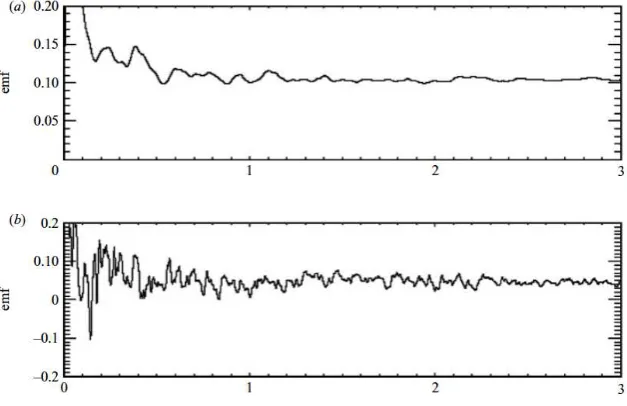
The issue of a potentially small value of the mean e.m.f. was addressed for rotating plane-layer convection by Hughes & Cattaneo (2008). They considered a regime in which the convection is turbulent, but still rotationally influenced, as revealed by the flow being noticeably helical. Figure 3 shows the time history of the longitudinal component of the spatially-averaged e.m.f. resulting from the imposition of a horizontal uniform field of strength B0 = 0.1 for convection at two different Rayleigh numbers (Ra = 80,000 and Ra = 150,000), with Taylor number T a= 500,000, Prandtl number P r = 1 and magnetic Prandtl numberP m= 5; the resulting Rossby numbers are Ro≈0.026 (Ra= 80,000) and Ro≈0.08 (Ra = 150,000). Figure 4 shows the corresponding cumulative averages. The imposed field is very weak, with B2
0/hu 2
i ≈2.8×10⁻⁵
for Ra= 80,000 and ≈ 3.1×10⁻⁶
for Ra = 150,000. At these parameter values the critical Rayleigh number for the onset of dynamo action is Ra ≈170,000; for the two cases shown, the e.m.f. is thus solely a result of the imposed field.
Figure 2.Field distortion by a localised helical disturbance. In (a) the loop is twisted through an angleπ/2 and the associated current is anti-parallel to B; in (b) the twist is 3π/2, and the associated current is parallel toB. (From Moffatt (1978).)
averaging a clear value of the mean e.m.f. (and hence α) eventually emerges. In the light of the preceding discussion, it is worth pointing out that the values ofαare small; in particular they are much smaller than a characteristic velocity: for Ra = 80,000,
α ≈ 1, whereas hu2 i1/2
≈20; for Ra = 150,000, α ≈0.4, whereas hu2 i1/2
≈ 60. For the case of Ra= 150,000 the long-time average value of αdiffers from a typical value (already spatially averaged) by a factor of 102
, which is O(Rm); thus, as a result of the incoherence of the e.m.f., its mean magnitude is determined by diffusive rather than dynamic processes. It has been argued that a much more healthy value of α can be attained if the mean field is ‘reset’ at regular short intervals (e.g. Hubbardet al. 2009); whereas this is true, since it implicitly adopts the short-sudden approach, the validity of the enhancedαis questionable. First, potentially important diffusive effects are reduced; furthermore, in the calculations of Hughes & Cattaneo (2008) described above, time averaging is simply seen as a proxy for spatial averaging, in that larger domains would require less temporal averaging; in this context the idea of ‘resetting’ cannot be justified (Hugheset al.2011).
3.4. Small-scale dynamo action
Figure 3.Time histories of the longitudinal component of the e.m.f. for rotating plane layer convection, with aspect ratioλ = 5,T a= 500,000,P r = 1,P m= 5, imposed field strength B0= 0.1 and (a)Ra= 80,000, (b)Ra= 150,000. (From Hughes & Cattaneo (2008).)
Figure 4.Cumulative averages of the longitudinal component of the e.m.f. as a function of averaging length, for the cases illustrated in Figure 3. (From Hughes & Cattaneo (2008).)
[image:11.493.93.407.310.513.2]values of Rm, act as dynamos, i.e. as (exponential) amplifiers of the magnetic energy. However the fields are small-scale — on the scale of the flow or smaller — with no significant large-scale component. The important question then arises as to where does the idea of small-scale dynamo action fit into the theory of mean field electrodynamics (see, for example, Boldyrevet al.2005, who considered this issue within the context of the Kazantsev dynamo). Partially to address this question we may consider the implications of small-scale dynamo action for the calculation ofαby the prescription outlined in§2.3. There are two issues to address: one is the practicable issue of calculation, the other is of interpretation; these are discussed in much more detail in Cattaneo & Hughes (2009). If the flow acts as a small-scale dynamo then for a uniform imposed field B0, the fluctuating field, and hence the e.m.f., grows exponentially. Even if measurable, this gives an α-effect that grows exponentially with time, which does not seem particularly helpful. In such a case one might instead considerB0 to be a large-scale component of the small-scale dynamo, in which case bothEandB0will grow exponentially at the same rate. The interpretation of the tensorsα andβ derived in this way is though certainly problematic, since, crucially, the growth rate of the observed field has nothing to do with that predicted by equation (2.11). A particularly striking example can be seen for the case of a non-helical dynamo. Here,αis zero and equation (2.11) therefore predicts that large-scale averages should decay exponentially at a scale-dependent rate. However, as we have just argued, any average of the small-scale dynamo will grow exponentially at the small-scale dynamo growth rate, with this growth rate being determined not from mean field dynamo considerations, such as lack of reflectional symmetry, but from small-scale dynamo considerations, such as stretching and constructive folding. For a helical flow, a true mean field dynamo would emerge as the only candidate at low Rm; at higher
Rmthis dynamo may still exist, but it would be unobserved since its growth would be swamped by the small-scale dynamo (see, for example, Shumaylovaet al. 2017).
4. The Dynamical Regime
Historically, mean field dynamo theory has resulted from consideration of the kinematic evolution of the magnetic field, i.e. that described by the induction equation for prescribed flows. However, in nature, there are no kinematic fields; the Lorentz force matters and the velocity and magnetic fields are related in a complex nonlinear fashion. It thus becomes important to consider how the mean field ideas of §3 can be extended into the nonlinear regime. There are, broadly, two ways in which one might do this. One, discussed in §4.1, which is closest in spirit to the original formulation, is to consider magnetohydrodynamic (as opposed to hydrodynamic) basic states and then to examine long wavelength instabilities of such states; this leads not only to extensions of existing mean field ideas, but also to new physical mechanisms, the implications of which have not yet been fully explored. The other, which we consider in§4.2, is to adopt the mean field ansatz (2.8), together possibly with a similar mean-field formulation for the velocity, and to calculate the dependence of the mean field tensors on the strength of the mean magnetic field (and flow).
4.1. Mean field instabilities of MHD states
of a small-scale dynamo, driven by some forcing F. Somewhat surprisingly, these ideas have been explored only fairly recently (Courvoisieret al.2010b,a).
In a pioneering paper of mean field electrodynamics, Roberts (1970) investigated the nature of the α-effect by considering the instability of spatially periodic hydrodynamic flows to long wavelength perturbations in the magnetic field. Courvoisier et al.(2010b) extended this idea to consider long wavelength perturbations to fully magnetohydrody-namic flows; crucially, in such an approach, the velocity and magnetic field, in both the basic state and the perturbations, are of equal significance. In brief, the idea is as follows. The starting point is a three-dimensional basic state B(x, t), U(x, t), which, for simplicity, we shall assume to be spatially and temporally periodic. We then consider long-wavelength perturbations, with wave vectork, of the form
(b(x, t),u(x, t)) = (H(x, t),V(x, t)) exp (ik·x+p(k)t), (4.1)
whereV andHvary on the same spatial and temporal scales as the basic state, andp(k) is thek-dependent growth rate of the perturbations. The wavelength of the perturbations, 2π/|k|, is assumed to be long in comparison with the spatial periodicity of the basic state. We now decompose the perturbations into average and fluctuating parts, with the average defined by
b,u
= (hHi,hVi) exp (ik·x+p(k)t), (4.2) where h i denotes an average over the spatial and temporal periodicities of the basic state;hHiand hVi are thus constants. The aim is to employ a mean field approach in order to determine the growth ratep(k) of modes with non-zero mean magnetic fields, i.e. modes for whichhHi 6=0.
The magnitude of the wave vectork=|k|is treated as a small parameter;H,V and the growth ratepare then expanded in powers ofk, so that, for example,
H=H0+H1+. . .Hn+. . . , (4.3)
whereHnis ofnthorder in the components ofk. At zeroth order, the governing equations
become
p0H0+ ∂t−Rm− 1
∇2
H0=∇×(V0×B+U×H0), (4.4)
p0V0+ ∂t−Re−
1 ∇2
V0=−∇Π0+∇·(H0B+BH0−V0U−U V0), (4.5)
∇·H0= 0, ∇·V0= 0, (4.6)
whereΠ denotes the perturbation to the pressure. Averaging equations (4.4) – (4.5) gives
p0hH0i=p0hV0i= 0. (4.7)
For non-zero mean field solutions we therefore need to takep0 = 0. The corresponding equations for the fluctuations are then
(∂t−Rm−1∇2)h0=∇×(v0×B+U×h0) +hH0i ·∇U− hV0i ·∇B, (4.8) (∂t−Re−
1 ∇2
)v0=−∇Π0+∇·(h0B+Bh0−v0U−U v0)
+hH0i ·∇B− hV0i ·∇U, (4.9)
∇·h0= 0, ∇·v0= 0. (4.10)
To first order, the equations for the mean variables give
p1hH0i=ik× hv0×B+U×h0i, (4.11)
It can be seen from equations (4.8) – (4.9) thath0andv0 are subject to a linear forcing by bothhH0iandhV0i. Therefore, expressions (4.11) and (4.12) can be rewritten as
p1hH0i=ik× αB· hH0i+αU· hV0i
, (4.14)
p1hV0i=−ikΠ0+ik· ΓB· hH0i+ΓU· hV0i
. (4.15)
The evolution of any long-wavelength instability to the magnetohydrodynamic basic state is thus governed by the four (constant) tensorsαB,αU,ΓBandΓU. These depend on the basic stateU,B, and hence on the forcing F and on the fluid and magnetic Reynolds numbers. For the kinematic dynamo problem, the only non-zero tensor is αB, which
reverts to the standardα-effect tensor. Similarly, for the mean field vortex instability — in the absence of magnetic field — the only non-zero tensor is ΓU, which describes
the anisotropic kinetic alpha (AKA) effect of Frisch et al. (1987). Finding a simple interpretation of these four tensors is even more difficult than for the purely kinematic problem, in which one has only the tensorαB. As in the kinematic case however, some progress can be made in the limit of small Rm (Courvoisier et al. 2010a); under this restriction, the (dimensionless) e.m.f. can be approximated at leading order by
λ2
R−1
mEi≈U0· h(1−P− 1
m )ǫijk∇ujbki
+B0· hǫijk(uj∇uk+Pm−1χ∇bjbk)i, (4.16)
where λis the monochromatic wavenumber of the forcing (in both the momentum and induction equations), χ is a dimensionless parameter related to the amplitudes of the forcings andP mis the magnetic Prandtl number. A related expression can be found for the mean stress in the momentum equation. Even in this simplest case, in which we have an explicit expression for the e.m.f. in terms of the field and flow, it should be recalled that it is the forcing that is prescribed and that the field and flow follow as fully nonlinear states of the MHD equations.
That said, it is of interest to note the form of theαB term (i.e. the coefficient ofB0) in expression (4.16). It involves both the flow helicityhu·∇×uiand the current helicity
µ−1
0 hb·∇×bi, and is reminiscent of the famous formula of Pouquetet al.(1976), namely
α=−τc 3
hu·∇×ui − 1
µ0ρ
hb·∇×bi
, (4.17)
derived by applying the EDQNM approximation to homogeneous, isotropic, helical MHD turbulence. It is tempting to regard (4.17) as a formula describing how the nonlinear saturation of a dynamo initially driven kinematically by the flow helicity is achieved through the counteracting build up of current helicity. However, as pointed out by Proctor (2003) (see also Blackman 2003), this temptation should be resisted. If, for simplicity, we make the short-sudden approximation, then the expression (3.4) forα, namely
α=−τc
3hu·∇×ui, (4.18)
Figure 5.(a) Growth rate and (b) frequency of the instability of an MHD basic state, determined both by the mean field approach (dashed line) and by a solution of the full instability problem (solid line). The basic state results from applying the AKA forcing with an imposed magnetic field;Rm= 16. (From Courvoisieret al.(2010b).)
order, by
∂u′
∂t =−∇p+
1
µ0ρ
B0·∇b, (4.19)
∂b′
∂t =B0·∇u. (4.20)
The e.m.f. is given, to leading order, by
E =hu×b′+u′×bi, (4.21)
from which expression (4.17) follows, on solving (4.19) and (4.20) foru′ and b′.
Finally we should consider the practicalities of evaluating the four tensorsαB,αU,ΓB
andΓU. In theory, they can be calculated by solving equations (4.11) – (4.13). Sometimes,
as in the standard determination ofα, everything works beautifully; similarly, sometimes it does not. Courvoisier et al. (2010b) extended the classic work of Roberts (1972) by considering two-dimensional magnetohydrodynamic states (dependent on x, y and t), attained by applying a forcing to a basic state with an imposed uniform field (attaining a two-dimensional MHD state via saturation of a dynamo is of course impossible). They then evaluated the four governing tensors and determined the resulting growth rate of an instability (of both field and flow) with a long wavelength in thezdirection. Furthermore, they could also solve the full instability problem independently and compare the two approaches. Figure 5 plots the real and imaginary parts of the growth rate, showing the comparison between the mean field approach and a full solution of the dynamo problem, for the case when the flow is forced by the AKA forcing of Frisch et al. (1987), with
Rm= 16. Since the mean field theory is performed to first order in wavenumberk, the associated growth rate is linearly dependent onk; the agreement for smallkis excellent. In all of the examples considered by Courvoisieret al.(2010b), it was straightforward to evaluate the governing tensors, with averages converging quickly. However, for three dimensional MHD states — and indeed possibly for two-dimensional states at higherRm
problem to that which undermines the determination of the kinematicα-effect in the case when a small-scale dynamo is present. However, we may then ask the question as to what happens if instead of imposing akinematicfield (or flow) we impose adynamicalmagnetic field, retaining the Lorentz force. Clearly, on energetic grounds, adding a very weak (but dynamic) magnetic field to an equilibrated MHD state will not lead to unbounded perturbations. The interesting question is whether, if the field is made sufficiently weak, there is indeed an e.m.f. that is linear in the imposed field — as assumed by the theory. In other words, can we salvage the linear theory in the circumstances for which the tensors are not calculable by considering the weak field limit of a dynamical field? This is clearly related to linear response theory (see, for example, Marconi et al. 2008), but the dependence of an averaged quantity to an external disturbance to a turbulent system is not necessarily straightforward (Hugheset al.2018).
4.2. Nonlinear mean field tensors: the quenching problem
A different approach to that outlined in §4.1 is to assume that, even in its dynamic state, the mean magnetic field still satisfies equation (2.9), but that all of the nonlinear effects are somehow incorporated into theαandβtensors. Attention has mainly focussed on the dependence of theα-effect on the mean fieldB0— what is known as the question of α-suppression or α-quenching. In dynamo models, one might also have a coupled mean field equation for the differential rotation, where the influence of the Reynolds stresses on the large scales results in what is known as aΛ-effect (R¨udiger 1989; R¨udiger & Hollerbach 2004). One can then also incorporate Λ-quenching. Here, since we are concentrating on the fundamental aspects of the mean field formulation, rather than looking at specific dynamo models, we shall restrict attention just to the suppression of the transport terms in the induction equation.
The idea of incorporating a dynamical element into the α-effect in order to prevent unlimited growth of the magnetic field is long standing (see Stix 1972; Jepps 1975). From an astrophysical perspective, the particular interest is in the nature of the suppression at very high values ofRm, and it is this issue that has led to some heated discussions over a number of years. At the heart of the matter is the question of how a magnetic field that is extremely weak on the large scales can, nonetheless, become dynamically significant on smaller scales. In a seminal paper, Vainshtein & Rosner (1991) proposed a mechanism by which an extremely weak large-scale magnetic field could suppress turbulent magnetic diffusion. More specifically, they argued that even if the energy in the large-scale field were as small as Rm−1
times the kinetic energy, then the associated small-scale field would be sufficiently strong to inhibit the turbulent diffusion process. These ideas were substantiated for the case of two-dimensional magnetohydrodynamic turbulence by the illuminating computations of Cattaneo & Vainshtein (1991) and Cattaneo (1994).
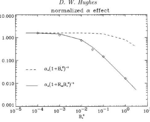
Figure 6. Normalised α-effect, αN = α33/hu 2
i, as a function of B2
0 for cases with
Rm=Re= 100. Each diamond corresponds to a numerical simulation. The dashed and solid curves are fits to the two different suppression formulae; in both cases the value atB2
0 = 10− 4
has been fitted exactly. (From Cattaneo & Hughes (1996).)
namely
α= α0 1 +B2
0/hu 2
i and α=
α0 1 +RmB2
0/hu 2
i, (4.22) with the value α0 determined from fitting α at the weakest field strength. In the former prescription, the magnetic field can reach equipartition strength before seriously influencing theα-effect; by contrast, in the latter, only a very weak large-scale magnetic field (of order Rm−1
times the kinetic energy) is needed to suppress α. It can be seen clearly from Figure 6 that the numerical results provide an excellent agreement with the more dramatic suppression formula. Clearly, if theα-effect is the dominant dynamo process in astrophysical contexts, in which Rm is invariably huge, then this dramatic suppression presents a major problem in explaining observed large-scale magnetic fields. It is though worth emphasising that the issue is one of suppression of the turbulent α -effect, i.e. in whichα0 ∼ hu2i1/2. In other words, anα-effect that acts on a fast (flow) timescale will be suppressed on that timescale. On a sufficiently long (Ohmic) timescale (though astrophysically this is extremely long), such suppression presents no impediment to the build up of strong large-scale fields (see, for example, Cattaneoet al. 2002; Bhat
et al.2016).
Despite strong numerical evidence for a strong (Rm-dependent) suppression of theα -effect, such as presented in Figure 6, together with underpinning theoretical arguments, this has proven to be a very controversial issue. Is the strong suppression a serious concern, or can it be sidestepped in some way? The strong suppression result of Cattaneo & Hughes (1996) was ascribed by Blackman & Field (2000) as being due to the adoption of periodic boundary conditions, and, in particular, to their influence on the magnetic helicity. Indeed, they go so far as to say that ‘this (the strong suppression result) is not a dynamical suppression from the back-reaction but a constraint on the magnitude ofα
designed to explore this issue have not yet been performed. Blackman & Field (2002) argue, somewhat differently, that the strong saturation result (4.22b) is valid only at very long times (on an Ohmic timescale), and that weaker suppression up to that time will allow significant field amplification. Although this is a possibility, it should be noted that in the simulations of Cattaneo & Hughes (1996), suppression is attained on a dynamical (fast) timescale.
Discussions on the saturation of theα-effect, together with the influence of boundaries, are often couched in terms of the magnetic helicity, defined by
HM =
Z
A·BdV, (4.23)
where Ais the magnetic vector potential, and where V is a volume bounded by a flux surface (i.e. a surface on which B ·n = 0) (Moffatt 1978). They are based on the twin notions that magnetic helicity is ‘almost conserved’ and that dynamos can be best understood through consideration of thefluxof magnetic helicity. The idea that magnetic helicity is ‘almost conserved’ was introduced in an extremely important paper by Taylor (1974), with the very specific aim of explaining the generation of reversed fields in toroidal plasmas. This conjecture by Taylor does not of course hold in all circumstances (nor indeed did Taylor claim that it would) but, nonetheless, it seems to have become part of dynamo folklore, leading to the idea that large-scale fields can prosper only through a flux of large-scale helicity (see, for example, Vishniac & Cho 2001). Both of these ideas are though somewhat troublesome. Magnetic helicity is not necessarily conserved, or indeed ‘almost conserved’, in a resistive fluid — certainly during any kinematic dynamo phase, the magnetic helicity, unless identically zero, grows at precisely the same rate as the magnetic energy. In addition, magnetic helicity, as in (4.23), is gauge invariant only when the volume V is bounded by a flux surface; the notion of a flux of magnetic helicity, a gauge-dependent quantity, from one scale to another, or through a boundary, is thus problematic. Although the notion of magnetic helicity can be extremely valuable in analysing the topology of magnetic field configurations (see, for example, Berger 1999), it is worth bearing in mind, particularly in the dynamo context, that it is not something over and above the magnetic induction equation: from a solution of the induction equation, the magnetic helicity necessarily follows.
5. Discussion
After a whistle-stop tour through the ups and downs of some fundamental aspects of the theory of mean field electrodynamics, we should reflect on where we stand — not just with the theory itself, but with the greater goal of explaining the maintenance of global-scale astrophysical magnetic fields. Somewhat oversimplifying matters, we may arrive at two very different viewpoints. On the one hand, it is certainly true that mean field models — none of which I have discussed in this review — are able to reproduce astrophysical magnetic fields extremely well; for example, it is possible to construct a mean field model, suitably parameterised, that has roughly periodic dynamo waves, propagating towards the equator, interspersed with intervals of greatly reduced activity — very much like the solar dynamo. Optimistically, one might therefore argue that, at heart, a mean field approach provides the appropriate framework for understanding astrophysical dynamos. Less optimistically, however, one might argue that the success of such models is due to the freedom allowed in the choice ofαij, βijk, etc. and that it is still extremely difficult
The most elemental problem we can consider in a mean field context is the kinematic growth of magnetic fields in a helical, turbulent flow at high Rm. In my view, here it seems that small-scale dynamo considerations (i.e. stretching, twisting and folding) will dominate over any mean field characteristics (such as helicity) and that any large-scale component of the field will simply be as part of the small-scale eigenfunction. As for possible mean field instabilities of a fully MHD basic state, this problem has not yet been fully explored. Pessimistically, there is the worry that any predicted mean field instability, deduced from an argument relying on separation of spatial scales, will not manifest itself in a system that actually has many intermediate degrees of freedom — rather than a long wavelength instability slowly emerging, as the theory would predict, it is conceivable that the basic state would simply adjust slightly to accommodate any perturbation.
Although maybe it is asking too much for large-scale fields to emerge solely from small-scale interactions (what would be termed an α2
-dynamo), this requirement is anyway unrealistic in astrophysical bodies, which, typically, have a global-scale flow. Incorporating a large-scale shearing flow into the mean field approach leads to what is known as an αω-dynamo: the toroidal field arises from the shearing of the poloidal component by the differential rotationω; theα-effect still has to close the dynamo loop by regenerating the poloidal field. Given some of the difficulties withαdiscussed in this review, we should consider how these might be allayed through the added ingredient of a global-scale shear flow or differential rotation. Within the mean field framework, one can envisage various possible beneficial effects of a velocity shear on the mean field dynamo process (see Hughes & Proctor 2009): for example, (i) that even though α is small, ω
is so effective that there may nonetheless be an effective αω-dynamo; (ii) more subtly, that the large spatial scale of the shear leads to an enhanced αthrough greater spatial correlation of the small-scale motions; (iii) that the anisotropy induced by the shear may lead to more exotic mean field effects (such as the shear-current effect of Rogachevskii & Kleeorin (2003)). Alternatively it may be that the answer lies outside the strictures of mean field theory.
Recently there have been various, rather different, studies to address this question through investigations of kinematic dynamo action driven by small-scale turbulence and a large-scale (imposed) shear flow. Yousefet al.(2008) showed how the combination of a shear flow with small-scale non-helical turbulence can lead to a large-scale magnetic field; here, interestingly, there is no conventionalα-effect and so the dynamo mechanism certainly lies outside the standard αω picture. Hughes & Proctor (2013) extended the plane layer rotating convection dynamo model of Cattaneo & Hughes (2006) by imposing a large-scale uni-directional horizontal shear flow, dependent only on the other horizontal component; hydrodynamic interactions between the convection and the shear lead to a flow with a broad range of scales. The presence of velocity shear both enhances the dynamo growth rate and also leads to the generation of significant magnetic field on the larger scales. However, by analysing spectrally filtered flows, it was shown that the dynamo depends crucially for its existence on the entire range of velocity scales, and that it could not be described in terms of a dynamo with scale separation. A somewhat different conclusion was reached by Cattaneo & Tobias (2014), who considered dynamo action driven by a combination of Galloway-Proctor cells (described by (3.5)), together with a much larger-scale steady shear flow. Here it was found that the shear could suppress the small-scale dynamo action, thereby allowing mean field processes to flourish, with the emergence of dynamo waves.
field, together possibly with the influence of other large-scale inhomogeneities, that further progress will be made. Whether the answer will be as elegant as classical mean field theory remains to be seen. Fifty years on, there is still some way to go!
I am grateful to STFC, who for many years have funded much of my own research on astrophysical dynamo theory.
REFERENCES
Berger, M. A. 1999 Introduction to magnetic helicity. Plasma Phys. Control. Fusion 41,
B167–B175.
Bhat, P., Subramanian, K. & Brandenburg, A.2016 A unified large/small-scale dynamo in helical turbulence.Mon. Not. R. Astron. Soc.461, 240–247.
Blackman, E. G.2003 Recent Developments in Magnetic Dynamo Theory. InTurbulence and Magnetic Fields in Astrophysics(ed. E. Falgarone & T. Passot),Lecture Notes in Physics, vol. 614, pp. 432–463. Springer-Verlag.
Blackman, E. G. & Field, G. B.2000 Constraints on the magnitude ofαin dynamo theory. Astrophys. J.534, 984–988.
Blackman, E. G. & Field, G. B.2002 New dynamical mean-field dynamo theory and closure approach.Phys. Rev. Lett.89, 265007.
Boldyrev, S., Cattaneo, F. & Rosner, R. 2005 Magnetic field generation in helical turbulence.Phys. Rev. Lett.95, 255001.
Cattaneo, F.1994 On the effects of a weak magnetic field on turbulent transport.Astrophys. J. 434, 200–205.
Cattaneo, F. & Hughes, D. W.1996 Nonlinear saturation of the turbulent αeffect.Phys. Rev. E 54, 4532.
Cattaneo, F. & Hughes, D. W.2006 Dynamo action in a rotating convective layer.J. Fluid Mech.553, 401–418.
Cattaneo, F. & Hughes, D. W.2009 Problems with kinematic mean field electrodynamics at high magnetic Reynolds numbers.Mon. Not. R. Astron. Soc.395, L48–L51.
Cattaneo, F., Hughes, D. W. & Thelen, J.-C.2002 The nonlinear properties of a large-scale dynamo driven by helical forcing.J. Fluid Mech.456, 219–237.
Cattaneo, F. & Tobias, S. M.2014 On large-scale dynamo action at high magnetic Reynolds number.Astrophys. J.789, 70.
Cattaneo, F. & Vainshtein, S. I.1991 Suppression of turbulent transport by a weak magnetic field.Astrophys. J.376, L21–L24.
Childress, S. & Gilbert, A. D.1995Stretch, Twist, Fold: The Fast Dynamo. Springer-Verlag. Courvoisier, A., Hughes, D. W. & Proctor, M. R. E.2010a A self-consistent treatment of the electromotive force in magnetohydrodynamics for large diffusivities.Astron. Nachr. 331, 667.
Courvoisier, A., Hughes, D. W. & Proctor, M. R. E. 2010b Self-consistent mean-field magnetohydrodynamics.Proc. R. Soc. Lond. Ser. A466, 583–601.
Courvoisier, A., Hughes, D. W. & Tobias, S. M.2006α-effect in a family of chaotic flows. Phys. Rev. Lett.96, 034503.
Cowling, T. G.1933 The magnetic field of sunspots.Mon. Not. R. Astron. Soc.94, 39–48.
Du, Y. & Ott, E.1993 Growth rates for fast kinematic dynamo instabilities of chaotic fluid flows. J. Fluid Mech.257, 265–288.
Frisch, U., She, Z. S. & Sulem, P. L.1987 Large-scale flow driven by the anisotropic kinetic alpha effect.Physica D 28, 382–392.
Galloway, D. J. & Proctor, M. R. E. 1992 Numerical calculations of fast dynamos in smooth velocity fields with realistic diffusion.Nature 356, 691–693.
Gruzinov, A. V. & Diamond, P. H.1994 Self-consistent theory of mean-field electrodynamics. Phys. Rev. Lett.72, 1651–1653.
Herreman, W. & Lesaffre, P.2011 Stokes drift dynamos.J. Fluid Mech.679, 32–57.
Herzenberg, A.1958 Geomagnetic dynamos.Phil. Trans. R. Soc. Lond. Ser. A250, 543–583.
imposed and dynamo-generated magnetic fields. Mon. Not. R. Astron. Soc 398, 1891–
1899.
Hughes, D. W. & Cattaneo, F. 2008 The alpha-effect in rotating convection: size matters. J. Fluid Mech.594, 445–461.
Hughes, D. W., Cattaneo, F. & Kim, E.-J.1996 Kinetic helicity, magnetic helicity and fast dynamo action.Phys. Lett. A223, 167–172.
Hughes, D. W., Mason, J., Proctor, M. R. E. & Rucklidge, A. M.2018 Nonlinear mean field MHD: how far can you get?(in preparation).
Hughes, D. W. & Proctor, M. R. E.2009 Large-scale dynamo action driven by velocity shear and rotating convection.Phys. Rev. Lett.102, 044501.
Hughes, D. W. & Proctor, M. R. E.2010 Turbulent magnetic diffusivity tensor for time-dependent mean fields.Phys. Rev. Lett.104, 024503.
Hughes, D. W. & Proctor, M. R. E. 2013 The effect of velocity shear on dynamo action due to rotating convection.J. Fluid Mech.717, 395–416.
Hughes, D. W., Proctor, M. R. E. & Cattaneo, F.2011 Theα-effect in rotating convection: a comparison of numerical simulations.Mon. Not. R. Astron. Soc.414, L45–L49.
Jepps, S. A.1975 Numerical models of hydromagnetic dynamos.J. Fluid Mech.67, 625–646.
Krause, F. & R¨adler, K.-H.1980Mean-Field Magnetohydrodynamics and Dynamo Theory. Pergamon.
Kulsrud, R. & Anderson, S.1992 The spectrum of random magnetic fields in the mean field dynamo theory of the galactic magnetic field.Astrophys. J.396, 606–630.
Larmor, J. 1919 How could a rotating body such as the Sun become a magnet? Rep. Brit. Assoc. Adv. Sci.pp. 159–160.
Marconi, U. M. B., Puglisi, A., Rondoni, L. & Vulpiani, A.2008 Fluctuation dissipation: Response theory in statistical physics.Phys. Rep.461, 111–195.
Moffatt, H. K.1978Magnetic Field Generation in Electrically Conducting Fluids. Cambridge University Press.
Moffatt, H. K. & Proctor, M. R. E. 1982 The role of the helicity spectrum function in turbulent dynamo theory.Geophys. Astrophys. Fluid Dyn.21, 265–283.
Parker, E. N.1955 Hydromagnetic dynamo models.Astrophys. J.122, 293.
Pouquet, A., Frisch, U. & L´eorat, J.1976 Strong MHD helical turbulence and the nonlinear dynamo effect.J. Fluid Mech.77, 321–354.
Proctor, M. R. E. 2003 Dynamo processes: the interaction of turbulence and magnetic fields. In Stellar Astrophysical Fluid Dynamics (ed. M. J. Thompson & J. Christensen-Dalsgaard), pp. 143–158. Cambridge University Press.
Roberts, G. O. 1970 Spatially periodic dynamos. Phil. Trans. R. Soc. Lond. Ser. A 266,
535–558.
Roberts, G. O.1972 Dynamo action of fluid motions with two-dimensional periodicity. Phil. Trans. R. Soc. Lond. Ser. A271, 411–454.
Roberts, P. H. 1994 Fundamentals of dynamo theory. In Lectures on Solar and Planetary Dynamos (ed. M. R. E. Proctor & A. D. Gilbert), p. 1. Cambridge University Press. Roberts, P. H. & Stix, M.1971 The Turbulent Dynamo: a translation of a series of papers
by F. Krause, K.-H. R¨adler, and M. Steenbeck.Tech. Rep.60. NCAR Tech. Note. Rogachevskii, I. & Kleeorin, N.2003 Electromotive force and large-scale magnetic dynamo
in a turbulent flow with a mean shear.Phys. Rev. E 68, 036301.
R¨udiger, G. 1989 Differential Rotation and Stellar Convection: Sun and Solar-type Stars. Taylor and Francis.
R¨udiger, G. & Hollerbach, R.2004The Magnetic Universe: Geophysical and Astrophysical Dynamo Theory. Wiley.
Shumaylova, V., Teed, R. J. & Proctor, M. R. E.2017 Large- to small-scale dynamo in domains of large aspect ratio: kinematic regime. Mon. Not. R. Astron. Soc.466, 3513–
3518.
Stix, M.1972 Non-linear dynamo waves.Astron. Astrophys.20, 9.
Taylor, J. B.1974 Relaxation of toroidal plasma and generation of reverse magnetic fields. Phys. Rev. Lett.33, 1139–1141.
Vainshtein, S. I. & Rosner, R.1991 On turbulent diffusion of magnetic fields and the loss of magnetic flux from stars.Astrophys. J.376, 199–203.
Vainshtein, S. I. & Zeldovich, Y. B. 1972 Origin of magnetic fields in astrophysics. Sov. Phys. Usp.15, 159–172.
Vishniac, E. T. & Cho, J.2001 Magnetic helicity conservation and astrophysical dynamos. Astrophys. J.550, 752–760.
Vladimirov, V. A.2012 Magnetohydrodynamic drift equations: from Langmuir circulations to magnetohydrodynamic dynamo?J. Fluid Mech.698, 51–61.